Lab 07

A first machine learning
species distribution model

Learning complex, non-linear patterns in environmental data

BIO597 Spatial Analysis of Biodiversity

Natural-history illustration of a wood frog beside a woodland pool in Maine.

Last week

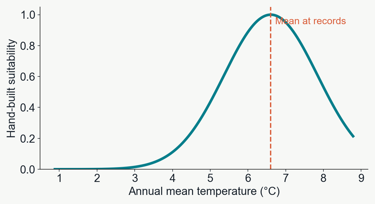
We chose the shape of the temperature response

Highest suitability near the mean temperature at records.

That was our assumption.

Today the model will learn a response curve, and it might not be very normal at all!

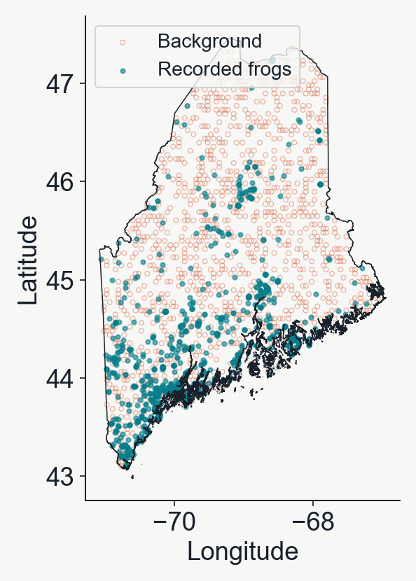
A hand-built suitability curve peaks at the mean annual temperature at complete wood-frog records.

The observations

Recorded environments and available environments

1 A frog record

0 A background sample

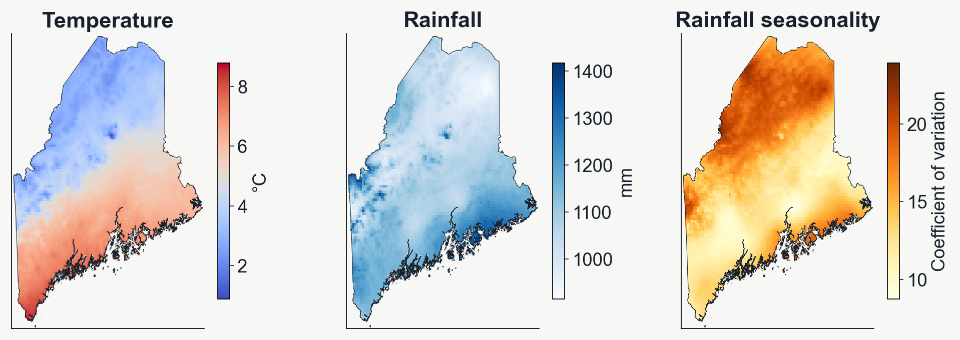
Background describes the climate available across Maine.

This is similar to what we did last week.

Maine map with teal wood-frog occurrence points and open coral background points sampled across the valid climate grid.

The input to the machine learning model is a table

Rows are occurrences or background points + environment

Climate columns are 'features' and the label column is the 'target'.

Temperature (°C)	Annual rainfall (mm)	Label
5.2	1,100	1 frog record
6.8	1,250	1 frog record
2.1	1,000	0 background
6.0	1,160	0 background

One decision tree

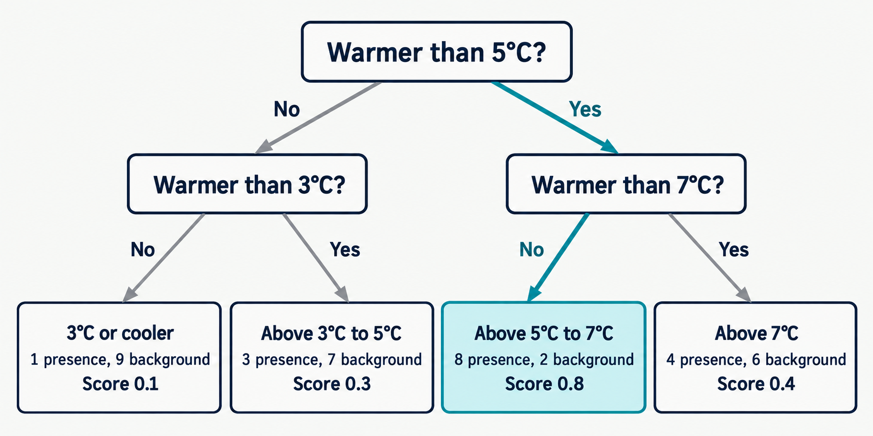
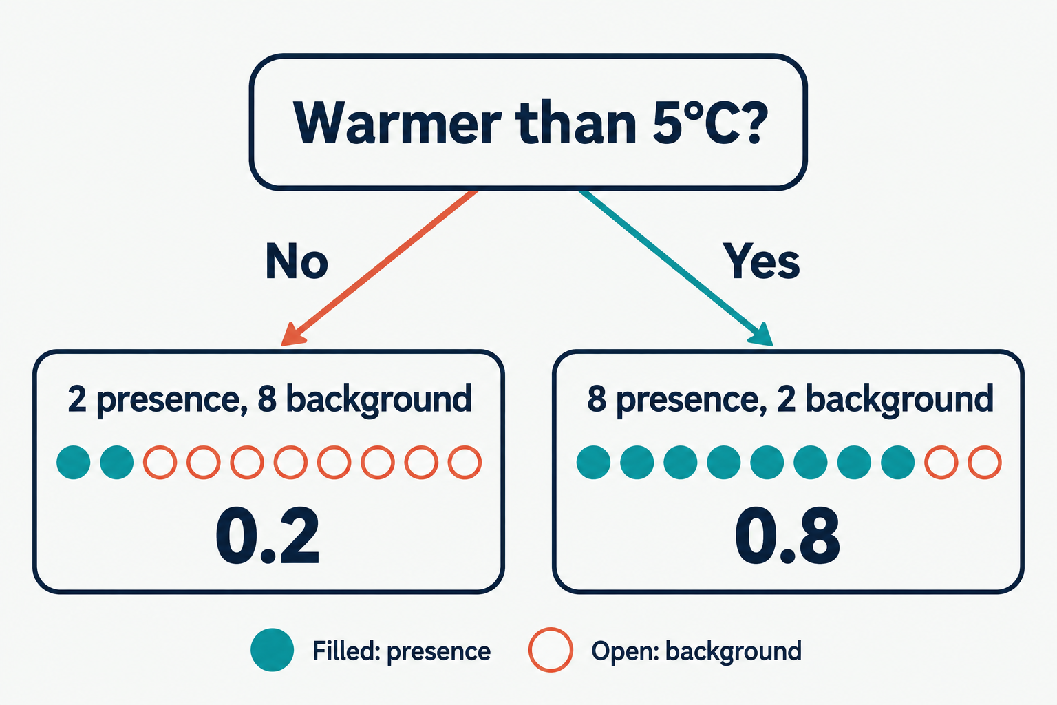
A question separates groups of examples

Within each final group, predict the average label.

There are, on average, more background points in the 'cold' class when the split is at 5 degrees C.

Illustration only. The model learns its own thresholds.

Illustrative decision tree asks whether temperature exceeds 5°C. The cooler group has 2 presence and 8 background labels, score 0.2. The warmer group has 8 presence and 2 background labels, score 0.8.

A deeper decision tree

Two levels of temperature splits

A depth-2 temperature decision tree splits first above 5°C, then above 3°C on the cooler branch and above 7°C on the warmer branch. The four final groups have scores 0.1, 0.3, 0.8, and 0.4. A highlighted path takes a 6°C location to the 0.8 group.

A 6°C location follows the highlighted path and receives a score of 0.8.

Depth 2 means two splits along each path.

Timing: 1.5 minutes. Start at the top with a hypothetical location whose annual mean temperature is 6°C. Is it warmer than 5°C? Yes, follow the right branch. Is it warmer than 7°C? No, follow the left branch into the group above 5°C and up to 7°C. That final group has eight presence labels and two background labels, so its mean label is 8/10 = 0.8. Ask students to trace 2°C, 4°C, and 8°C, which end at scores 0.1, 0.3, and 0.4. Depth counts the number of splits from root to final group: the root is depth 0, its child questions are depth 1, and the four final groups are depth 2. The tree uses temperature repeatedly, so one predictor can produce several different scores and a response that rises and then falls. All thresholds, counts, and scores are invented to illustrate the mechanism, not fitted to the wood-frog data. Source: https://scikit-learn.org/stable/modules/tree.html. Diagram generated for this lecture; see assets/Lecture07-artwork-notes.md.

A fitted tree

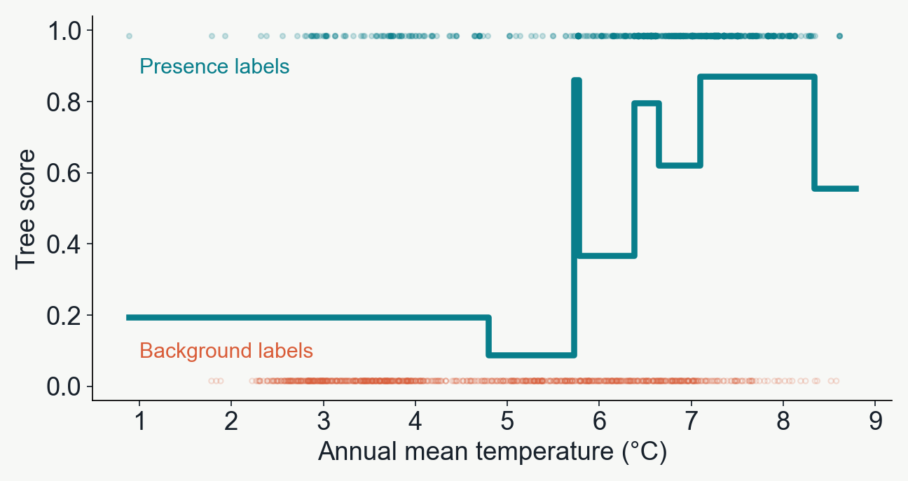
Decision tree predictions take on a step-shaped response

A small fitted decision tree gives a step-shaped score across annual mean temperature. Teal marks show presence labels and open coral marks show background labels.

The group boundaries come from the training data.

A random forest

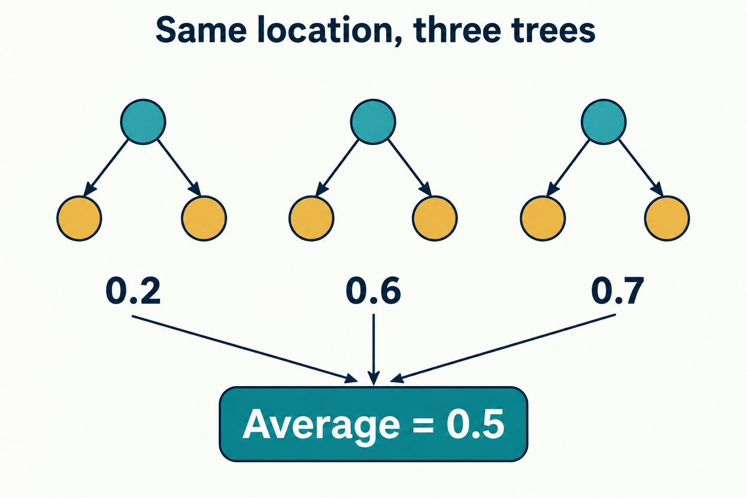
Many trees contribute to one score

Each tree learns from a different resample of the training records.

The forest averages their scores.

Three trees shown here. The lab uses 100.

Illustrative scores of 0.2, 0.6, and 0.7 from three trees average to a forest score of 0.5.

Model validation

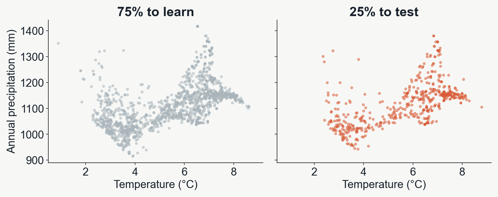
The use of training vs testing sets

Two plots in temperature and precipitation space show the 75 percent training sample in gray and the 25 percent held-out test sample in coral.

Test data is withheld during training and used to evaluate model performance on 'unobserved' data.

The standard scikit-learn API

Learn a relationship, then apply it

.fit()

Learn the mapping from environment ('features') to presence/absence ('targets').

.predict()

Predict presence/absence for environment of test-set and compare to known test-set labels.

model.fit(X_train, y_train)

scores = model.predict(X_test)

X = selected climate columns
y = presence/background labels

Evaluating predictions

Error is the distance from the assigned label

Known label	Prediction score	Absolute error
1 frog record	0.8	0.2
0 background	0.3	0.3
1 frog record	0.4	0.6

Average error = (0.2 + 0.3 + 0.6) / 3 ≈ 0.37

Mean absolute error (MAE). Lower is better.

Scaling to more predictors

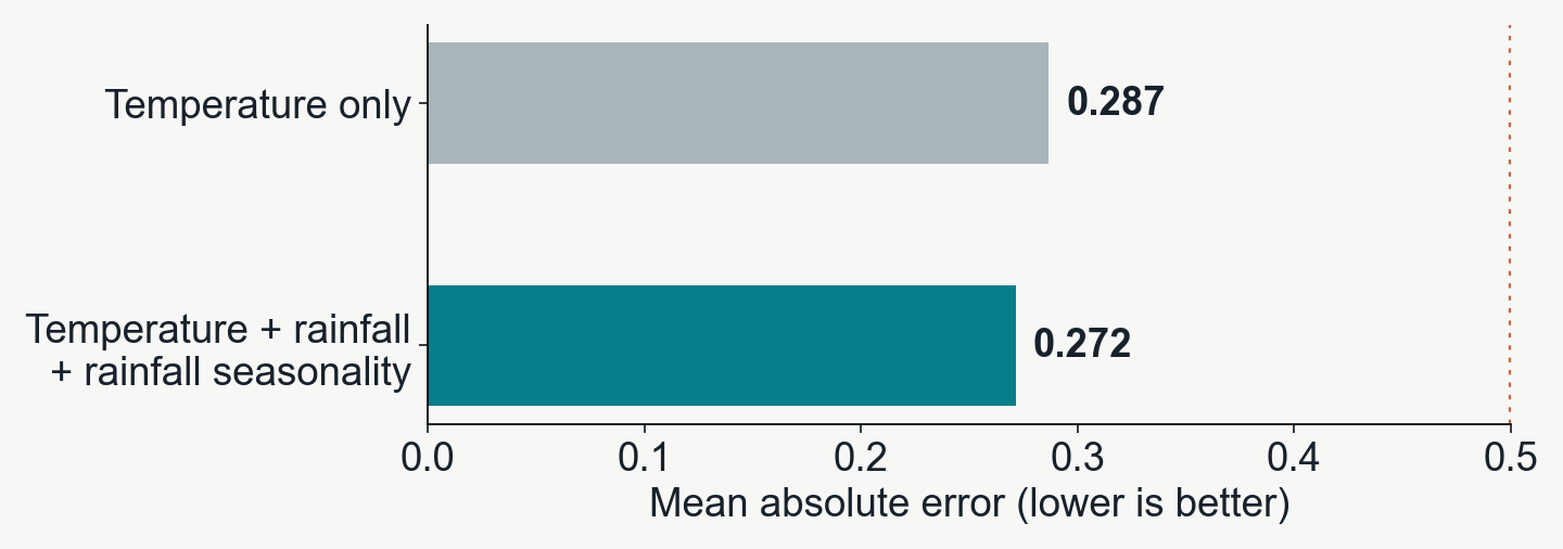
Does adding more features (more predictors) add useful information?

Three Maine raster maps show annual mean temperature, annual precipitation, and precipitation seasonality, with units on color scales.

Would two places with similar temperature always suit a frog equally well? What if one was super arid and the other humid?

The comparison

Temperature alone versus three climate variables

In one reproducible wood-frog example, temperature-only MAE is 0.287, compared with 0.272 after adding annual rainfall and rainfall seasonality.

In this example, precipitation reduces test error, but this isn't necessarily always the case.

Projection

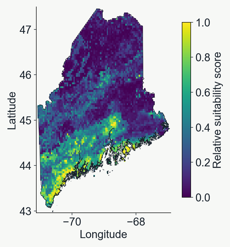
Running 'predict()' function across the landscape

Once the ML model is fit to the data, you can use the 'predict()' function to project suitability.

Extract the 3 fitted bioclim variables at each cell of the raster.

A high score means climate is more suitable (under this model).

Maine relative suitability map from the all-data three-variable wood-frog random forest, ranging from 0 to 1.

Variable importance

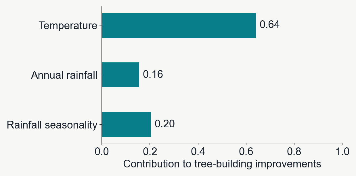
Which variables helped the trees separate labels?

Horizontal bars show training-based importance for temperature, annual rainfall, and rainfall seasonality in the final three-variable forest.

Not all variables contribute equally. Variable importance isn't necessarily _explanatory_, it is correlated though.