Lab 08

MaxEnt and spatial model evaluation

Introducing a few more advanced SDM concepts

BIO597 Spatial Analysis of Biodiversity

Natural-history illustration of a pickerel frog on a mossy bank beside a Maine woodland stream.

This week

A classic presence/background model

Approach	How the relationship is built
Our first SDM	We chose a simple temperature curve.
Random forest	ML learned a mapping between env correlates and presence/absence.
MaxEnt	A classical statistical model for fitting presence data to environmental evidence.

A foundational MaxEnt SDM paper: Phillips, Anderson & Schapire (2006).

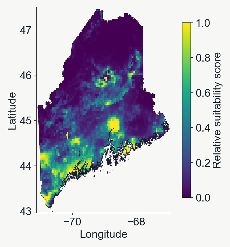
A real MaxEnt fit

MaxEnt prediction projected across the landscape

Just like our previous examples, the fitted MaxEnt model can be used to predict suitability at unobserved locations.

Internally, a penalty discourages unnecessarily complex responses.

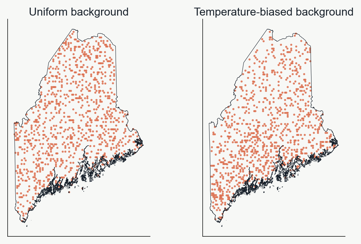
Relative suitability map for pickerel frogs fitted with elapid MaxentModel using 19 climate rasters and weighted presence/background records.

Accounting for observation bias when sampling background points

The background can influence the predictions

Two actual Maine background samples compare uniform sampling with sampling that favors warmer annual-mean-temperature cells.

Observations will be biased toward where humans usually go (near roads, in parks, where they think the organism will be), so it's important to replicate this bias as much as possible when sampling background points.

In the lab we will take mean annual temperature as a proxy for sampling bias, but in practice you might do something fancier.

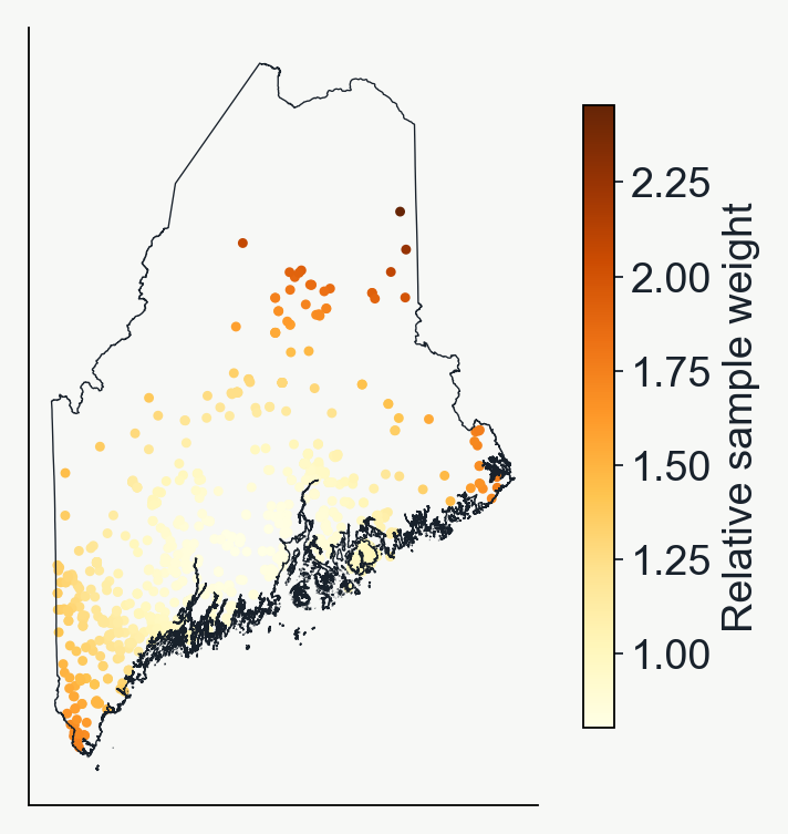
Geographic sample weights

Sample weights change a point’s influence

Many neighboring observations can repeat similar information.

Distance-based weights give relatively isolated records more influence.

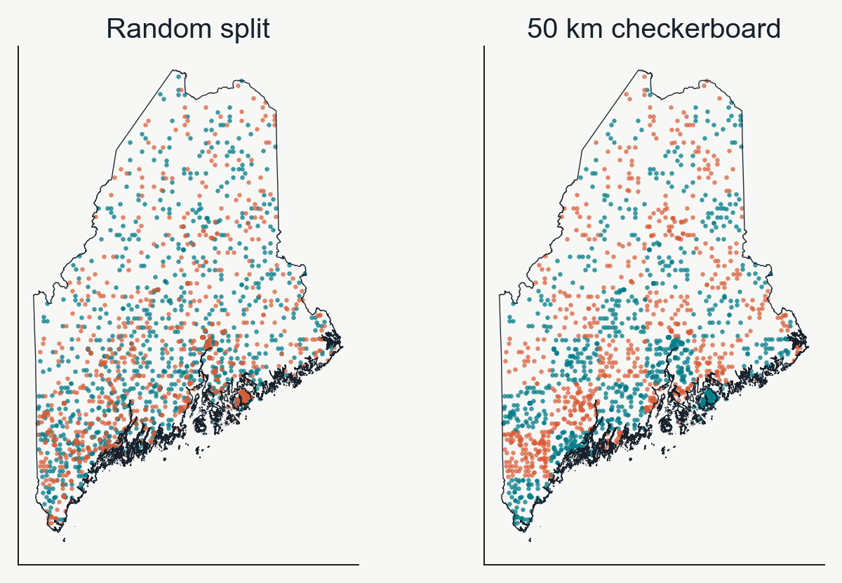
Pickerel-frog occurrences colored by distance-based sample weight, calculated in projected meters using elapid distance_weights.

Geographically aware splitting

Geographic splits withhold whole blocks

Keep an entire square in training or testing.

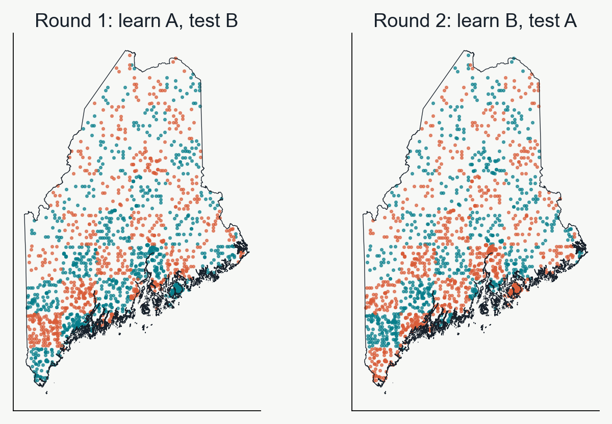
Lab08 uses alternating 50 km squares.

Teal training set. Coral test set. Nearby locations often share climate and sampling history.

Actual elapid checkerboard split of Maine modeling points, with entire 50 km blocks assigned to training in teal or testing in coral.

Evaluating robustness of test/train splits

Cross-validation rotates the test group

Presence/background points are split into 'K-fold' groups, and each group takes a turn as the withheld data. A new model is fit to each 'fold' of the data, and performance is evaluated as the average across N-folds.

	Group A	Group B	Group C
Round 1	Test	Train	Train
Round 2	Train	Test	Train
Round 3	Train	Train	Test

A group is often called a “fold.”

Two-fold spatial cross-validation

The checkerboard groups can swap roles

Two rounds swap the training and test roles of the same two checkerboard groups. The geometry and background sample stay fixed.

Each model predicts the group of locations it did not use for learning.

Leave-one-out (LOO) cross-validation is the logical extreme of k-fold

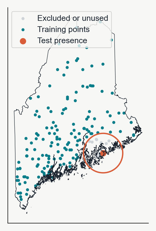
Buffered LOO controls for spatial auto-correlation

Hold out one observation as the test data.

Remove training points within 50 km.

Fit the SDM to all the remaining points.

Evaluate prediction accuracy for the one held-out point.

Repeat for another observation.

A held-out presence in coral has a 50 km exclusion circle. Training points outside the circle remain teal and excluded points appear gray.

Evaluating the frog model

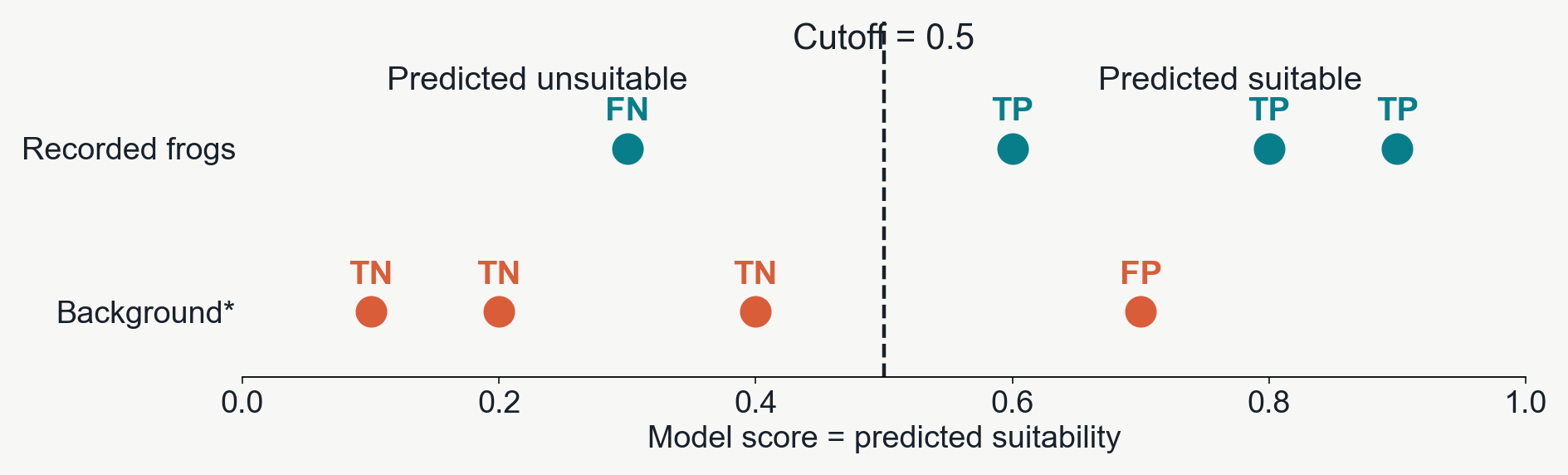
Which sites does the model call suitable?

A cutoff at suitability score 0.5 separates predicted unsuitable from predicted suitable sites. Three recorded frogs lie above the cutoff, labeled TP, and one below, labeled FN. One background site lies above the cutoff, labeled FP, and three below, labeled TN.

True positives (TP): recorded frogs predicted suitable — 3 of 4.
False positives (FP): background sites predicted suitable — 1 of 4.

*For presence/background AUC, background serves as the “negative” class. These are not confirmed absences.

Timing: 1.5 minutes. Lead with the figure. Each dot is a location and its horizontal position is the model’s predicted suitability, or score. Higher means more suitable under the model, not a calibrated probability of occurrence. The cutoff turns this continuous prediction into a positive (suitable) or negative (unsuitable) label. At 0.5, three of four recorded frogs qualify: true-positive rate 75%. One of four background sites qualifies: false-positive rate 25%, using background as the negative class. FN means a recorded frog predicted unsuitable, a missed presence. TN means a background site predicted unsuitable. Ask students to imagine sliding the dashed cutoff to the left: more sites qualify, increasing the fractions of true and false positives. This change traces the ROC curve on the next slide. These eight predictions are invented to teach the calculation. With confirmed absence data, a false positive would mean predicting suitable at an observed absence. Here background occupancy is unknown, so “false positive” is a conventional evaluation label, not a demonstrated ecological mistake. Source: https://scikit-learn.org/stable/modules/generated/sklearn.metrics.roc_curve.html.

Comparing models across all cutoffs

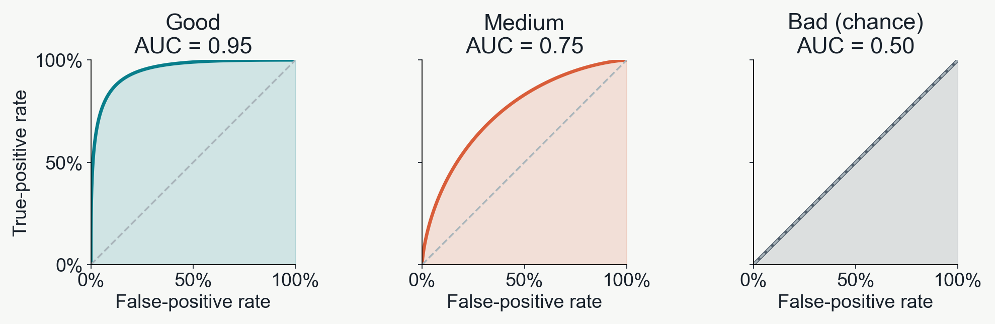
Good predictions find frogs with fewer false alarms

Three illustrative ROC panels labeled Good, Medium and Bad (chance), with shaded AUC values 0.95, 0.75 and 0.50. Each plots true-positive rate against false-positive rate. The good curve approaches the upper-left corner, the medium curve bends moderately above the diagonal, and the bad curve follows the chance diagonal.

Moving the cutoff traces each ROC curve. Toward the upper left: more true positives, fewer false positives.

AUC = area under the curve. Larger areas mean better separation of recorded frogs from background.

Illustrative curves, not fitted results. “Good,” “medium” and “bad” describe these examples, not universal AUC thresholds.

Timing: 1.5 minutes. Lead with the three panels. The vertical axis is the fraction of recorded frogs predicted suitable (true-positive rate, TP divided by TP plus FN). The horizontal axis is the fraction of background sites predicted suitable (false-positive rate, FP divided by FP plus TN). Every cutoff supplies one pair of rates. A good curve rises steeply: we recover many frogs before labeling much background suitable. The medium model needs more false positives to recover the same fraction of frogs. The bad example follows the diagonal: its predictions separate recorded sites and background no better than chance. The shaded area summarizes the curve, ranging from zero to one. Perfect separation gives AUC 1; chance ordering gives 0.5; systematically reversed predictions can fall below 0.5. AUC does not mean the percent of sites correctly classified or the probability of finding a frog. These are smooth theoretical curves with analytically known AUCs of 0.95, 0.75 and 0.50, not the course model’s results or universal grading categories. AUC depends on the test locations and sampled background, leading into the next slide’s random/spatial comparison. Background serves as the negative class here, rather than confirmed absences. Reproducible figures: assets/Lecture08-build-figures.py. Source: https://scikit-learn.org/stable/modules/generated/sklearn.metrics.roc_curve.html.

High AUC isn't always 'better'

Spatially/environmentally informed splits can improve model generalizability

Evaluate using	AUC	What is the model predicting?
Training records	0.875	Locations it already learned from
A random test split	0.798	Held-out points, often near training points
A spatial test split	0.664	Entire withheld geographic blocks

A higher random-test AUC can reflect an easier test, rather than better prediction in new areas.

Nearby points share climate and local patterns. Spatial splits reduce this overlap and help expose overfitting to those patterns.

Timing: 2 minutes. Distinguish suitability scores at individual sites from AUC, which summarizes how well a set of those scores separates recorded and background sites. The table contains actual fitted results, not the six-point teaching example. Training AUC uses the fitting data and can be optimistic. Random holdouts can remain spatially similar to training points, allowing a model to benefit from shared local conditions or sampling patterns. Withholding geographic blocks reduces this dependence and asks a harder question about prediction in other areas. A lower spatial AUC can expose reliance on local patterns that fails to generalize, including spatial overfitting. Spatial evaluation does not itself remove overfitting from the fitted model; using spatial validation to choose predictors or model complexity can help select models that generalize. Appropriate block size matters, and adjacent checkerboard blocks do not guarantee complete independence. Spatial splits can also withhold unfamiliar climates. Thus this AUC gap alone cannot identify its cause, prove overfitting, or establish that every spatial split is better for every prediction goal. Fit details: 1007 annotated presences, 908 biased-background points, distance weights and 19 predictors. Two checkerboard boundary rows are omitted. Random and checkerboard A-to-B fits use the same eligible pool and equal train/test sizes, 1136 and 777. The training-row fit uses all 1913 eligible rows and evaluates on them. Reverse checkerboard AUC is 0.789, illustrating regional variation. Full settings: assets/Lecture08-example-results.json. Sources: https://doi.org/10.1111/ecog.02881 and assets/Lecture08-build-figures.py.

Sources and visual credits