Lab 09 · October 30, 2026

Gradient Forest

From species distributions to genomic turnover

Where along an environmental gradient does genetic composition change?

BIO597 Spatial Analysis of Biodiversity
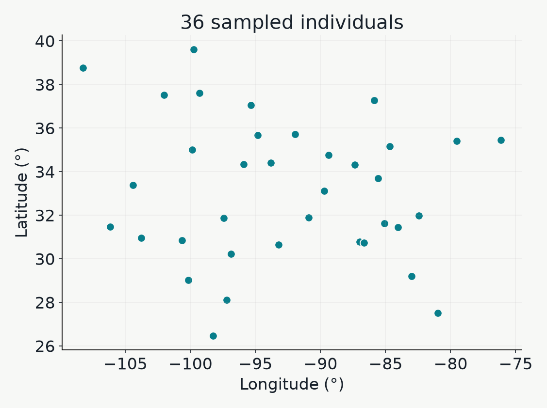
Longitude and latitude of the 36 P. guttatus individuals in the pyGF example. These points describe sampling, not the species range.

Points are sampled individuals.

Correlations between environmental predictors and genetic data

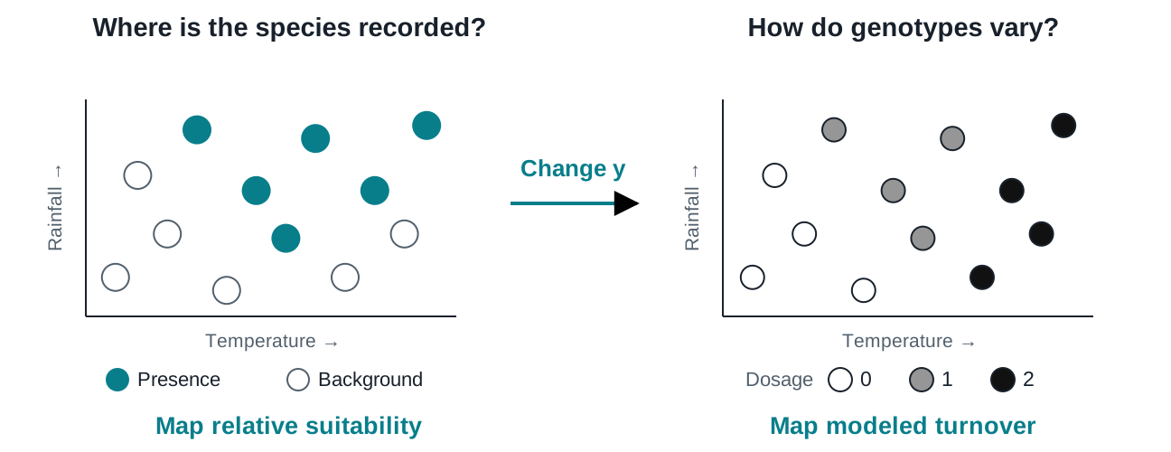
Same climate (predictor) but a different response (SNPs).

Two environmental scatterplots contrast presence/background labels with white, gray and black individual SNP dosages.

Keep the environmental predictors; replace occurrence labels with SNP dosages.

Encoding genotype data into a compact format

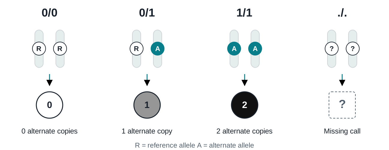
Count the alternate copies

Paired chromosome cartoons show reference/reference, reference/alternate and alternate/alternate becoming white zero, gray one and black two. Missing calls use a dashed box and question mark.

Two chromosome copies give a dosage of 0, 1, or 2.

Thinking about filtering/QC

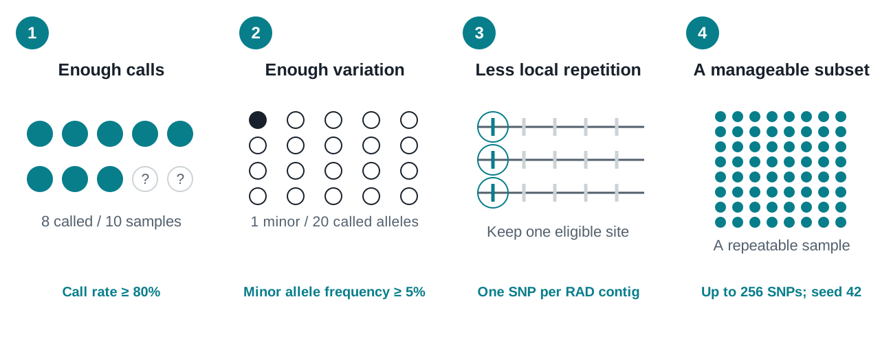
Filter for missingness, sufficiently variable sites, LD, and take a subset so it runs faster.

Four cartoons illustrate eight called samples out of ten, one minor allele among twenty called copies, one highlighted SNP per RAD contig, and a repeatable subset of loci.

Filtering chooses which genetic variation enters the analysis.

The gradient forest model

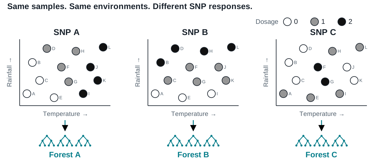
One random forest for each SNP

Three temperature–rainfall plots show the same twelve samples A through L at identical environmental positions. White, gray and black points encode dosages zero, one and two at SNP A, B and C. Each SNP panel feeds its own separate random forest.

Each forest sees the same environments and learns one SNP’s dosage pattern.

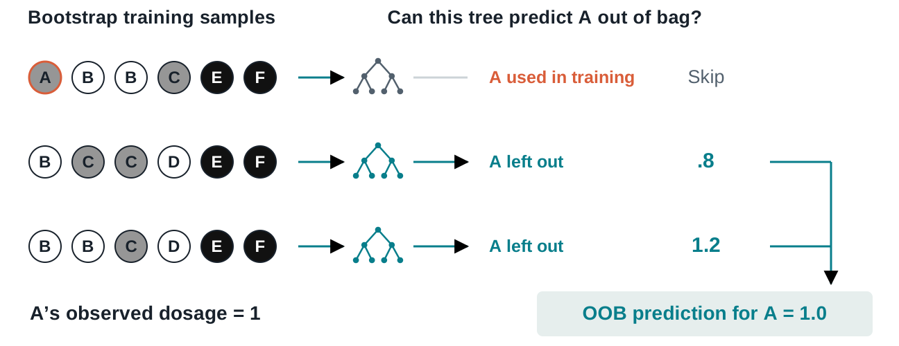
"Out of bag" prediction error

Evaluating ability to predict genotype of holdout set of samples

Three bootstrap samples feed three trees. The first includes A and is skipped; two exclude A and predict 0.8 and 1.2, averaging to an OOB dosage prediction of one.

Average predictions from trees that never learned from individual A.

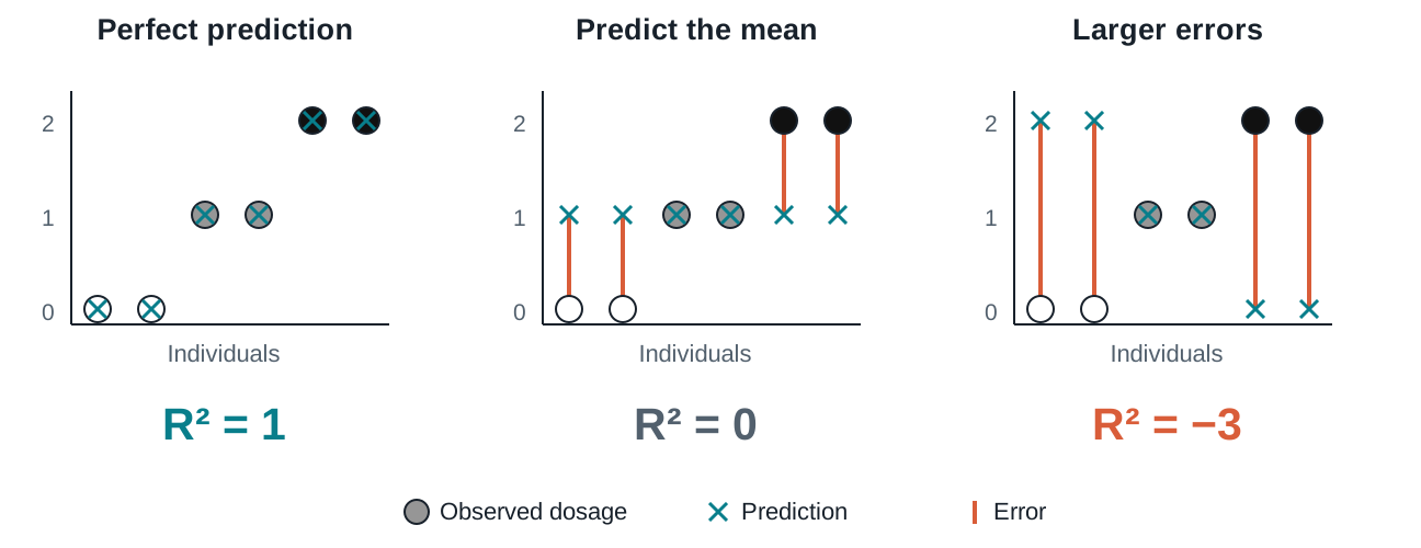
Evaluating model fit

Aggregating OOB prediction error across all Trees/SNPs

Observed genotype dots and prediction crosses compare perfect predictions, constant-mean predictions, and reversed predictions. Their R squared values are one, zero, and minus three.

R² = 0 matches the mean-only benchmark; positive scores improve on it.

The fitted example

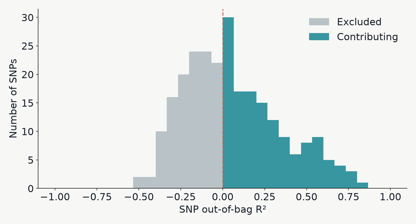
Some SNPs contribute; others do not

Histogram of fitted SNP OOB R squared values. Gray marks excluded responses and teal marks responses retained in the turnover summary; the dashed line marks zero.

pyGF retains SNPs with positive OOB R² and positive permutation importance.

Evaluating climate variable importance

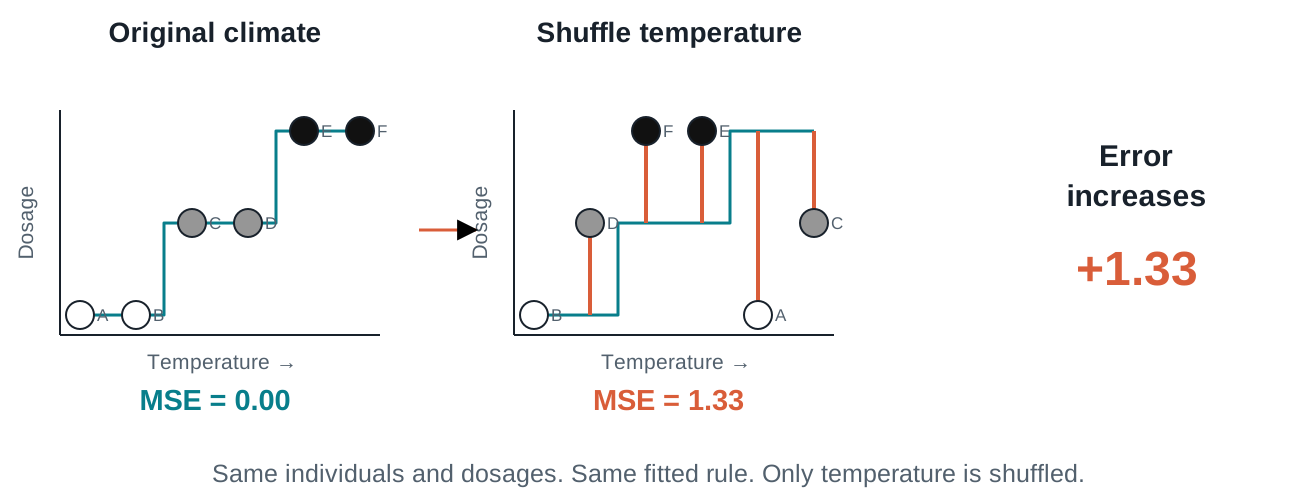
Shuffle climate; see what breaks

The same six individuals have unchanged dosage values but shuffled temperature values. A fixed step prediction rule then makes larger errors, increasing mean squared error from zero to 1.33.

If prediction error grows, the fitted forest relied on that variable.

Combining the forests

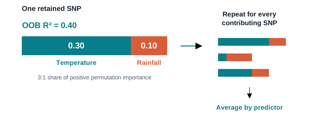
Share useful signal among the predictors

A bar totaling OOB R squared 0.4 is divided into temperature 0.3 and rainfall 0.1. Separate bars for other SNPs are combined by averaging each predictor allocation.

Give predictors a share of each SNP’s OOB prediction accuracy, then average over contributing SNPs.

The fitted example

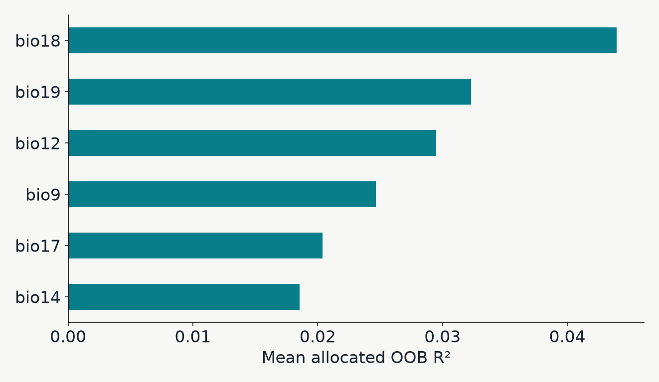
Which gradients carry the most modeled signal?

The six highest-ranked climate predictors by mean allocated out-of-bag R squared in the actual P. guttatus example fit.

BIO18 leads: precipitation of the warmest quarter.

From trees to gradients

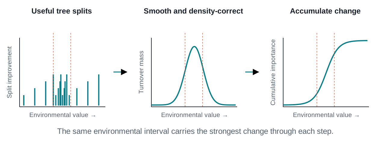
From useful splits to a turnover curve

Three aligned environmental axes show useful split locations clustering in the middle, a smoothed density-corrected turnover peak, and a cumulative curve rising most steeply over the same interval.

A cluster of informative splits becomes a steep part of the cumulative curve.

Schematic shapes. Smoothing and density correction account for where samples fall along the gradient.

The fitted example

Read the location and magnitude of turnover

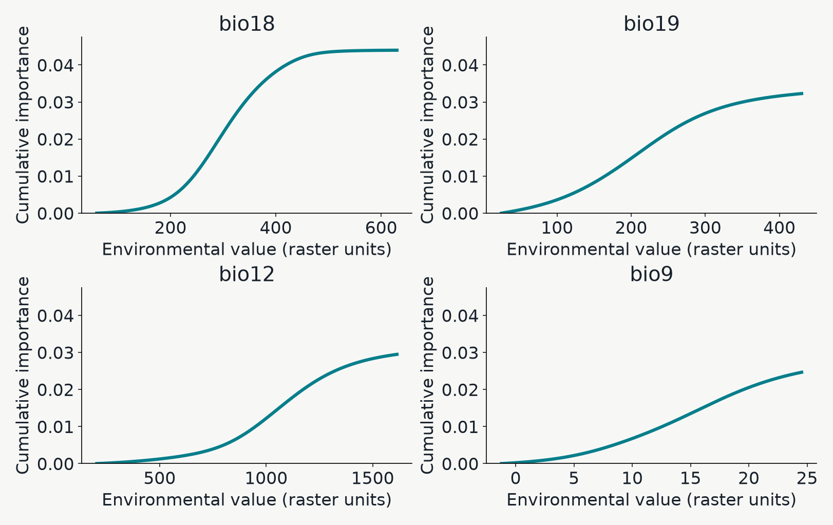
Cumulative turnover curves for the four most important fitted climate variables. Each curve has a nondecreasing shape and an endpoint equal to its mean allocated importance.

Steep segment: faster modeled turnover. Endpoint: total predictor importance. X axes retain each raster’s units.

A new environmental coordinate system

Stretch climate space where turnover is fastest

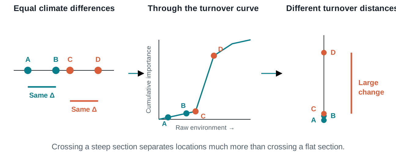
Two equal differences on an environmental ruler pass through a cumulative curve. A and B remain close on the transformed scale, while C and D span the steep rise and become widely separated.

The same raw climate difference can become a small or large turnover distance.

Illustration. In pyGF, transform() and predict() return these turnover coordinates.

Project across the landscape

A turnover layer is a transformed climate surface

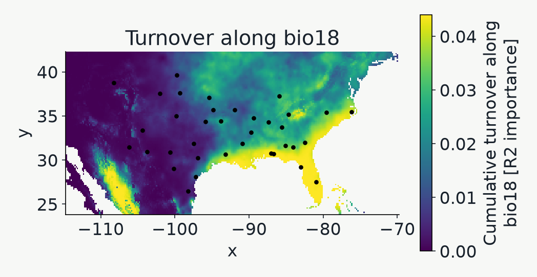
Regional map of the highest-ranked predictor after transformation through its cumulative turnover curve, with sampled individuals overlaid.

gf.plot_turnover() selects the leading predictor. High values mark cumulative position along that gradient.

Summarizing nineteen turnover coordinates

PCA gives the map and biplot a shared color key

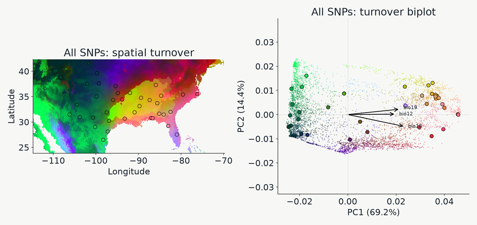
Actual regional map and PCA biplot of GF-transformed environments. Map locations and ordination points share RGB colors derived from the first three principal components.

PC1/2 locate biplot points. PC1/2/3 supply RGB colors. Similar colors indicate similar displayed coordinates.

Reading the biplot

Read the biplot as an environmental compass

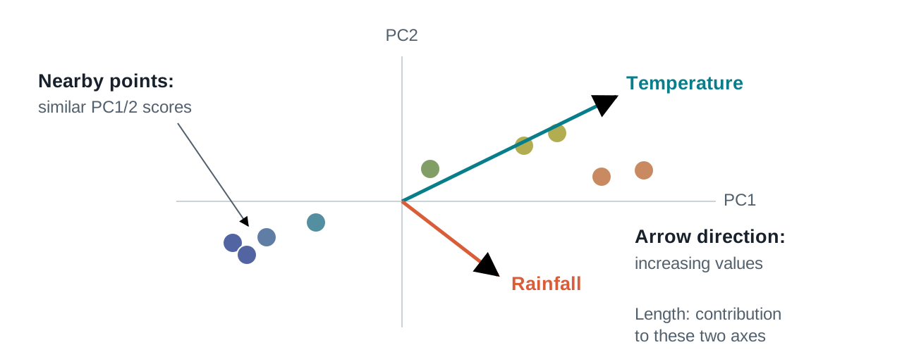
An enlarged PCA scatterplot shows nearby similarly colored points and two environmental arrows starting at the origin, with annotations for direction and contribution.

Follow an arrow toward increasing transformed values; compare its contribution to PC1/2.

Schematic PCA scores and covariance arrows. Nearby points share similar scores on the displayed axes.

Aggregate versus one locus

A single SNP can emphasize a different pattern

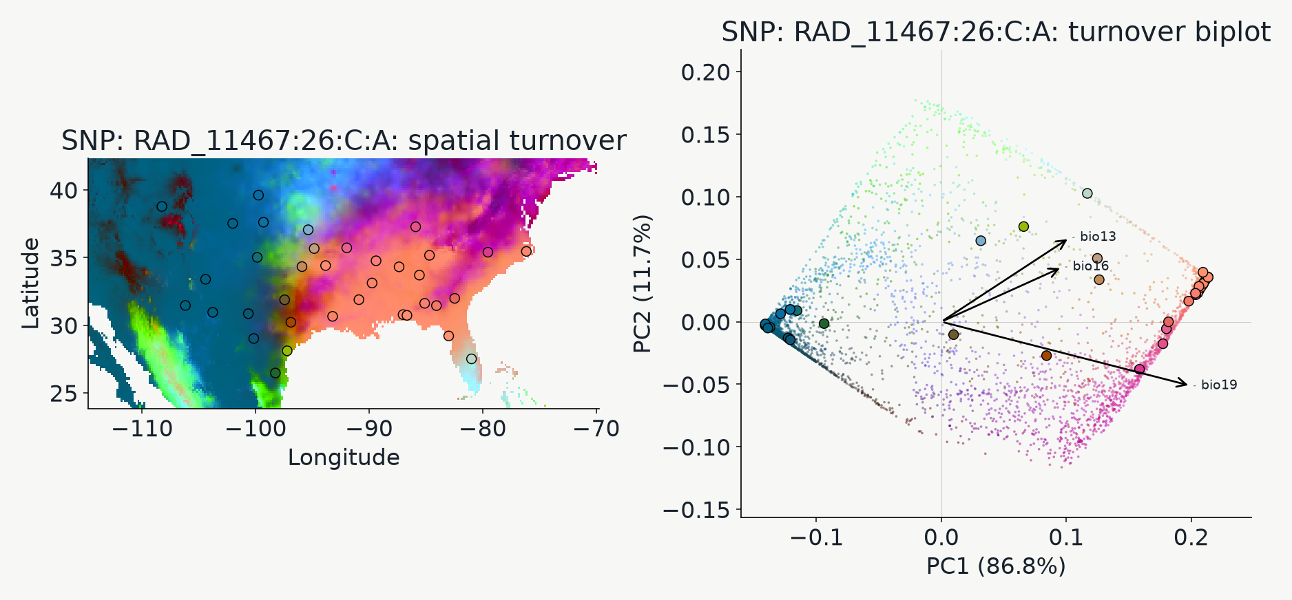
PCA map and biplot based on turnover curves of the SNP with the highest fitted OOB R squared, using its own PCA and RGB calibration.

Single-SNP view: response=snp. Each view has its own PCA basis and color scale.

Biological interpretation

The same pattern can have different explanations

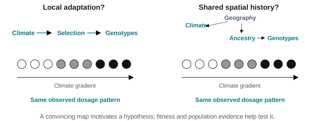
Two identical white-to-gray-to-black genotype gradients illustrate local adaptation as one hypothesis and shared geography and ancestry as another route to the same observed association.

A climate–genotype association gives us a hypothesis to test.

Conceptual alternatives. Fitness measurements and population-history evidence help distinguish them.

Sources and figure provenance

Further reading

pyGF is an independent implementation; conditional permutations and smoothing differ from R gradientForest.