Lab 10 · November 6, 2026
Community composition
Today you are a hypothetical land manager with a mission to conserve biodiversity.
How do we quantify spatial biodiversity patterns to answer questions about conservation?
BIO597 Spatial Analysis of Biodiversity
Allow about 45–50 minutes with discussion, or move quickly through the worked calculations for a shorter introduction. Students have mapped occurrence points and modeled distributions. Today the response becomes an entire community, and the conservation question determines which summary matters. The map is generated from the current ME_ImaginaryParks.geojson; it is not a map of real protected areas. All subsequent animal-icon examples and counts are invented unless explicitly labeled as lab data. Press S for presenter notes. Figure provenance and rebuild instructions are linked at the end.
The organizing question
Single Large or Several Small: SLOSS
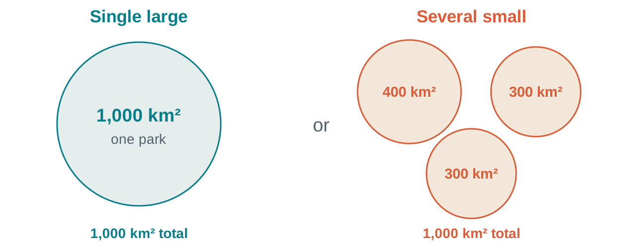
Equal area gives us a comparison. There is still huge debate about the right strategy.
A long-running conservation debate: Simberloff & Abele (1976) .
Ask for a show of hands before introducing any metric. What assumptions motivated each choice? Larger continuous habitat may support processes and populations that small patches cannot; separated reserves may capture different environments and species. These are hypotheses to evaluate, rather than universal rules. Simberloff and Abele challenged the inference that one largest possible refuge must always be best. This lecture does not settle the broader fragmentation debate. The three circle areas sum exactly to the large circle area; distances and habitat quality in this schematic have no quantitative meaning.
Define the conservation objective
“More biodiversity” can mean several things
If the goal is… We need to examine…
Conserve more species Species richness Avoid dominance by a few species Abundance distributions (Entropy and evenness) Capture different communities Beta diversity (turnover) Protect rare species Endemism and range information
Identify the conservation goal before choosing the focal biodiversity index.
These objectives overlap but can rank sites differently. Species identity matters as well: a network can be species rich while missing a focal threatened species. High Shannon diversity is not inherently the goal of every conservation program. A naturally dominated community can still be valuable. Today we will make each measure concrete and use differences among measures to ask better biological questions. Demographic persistence, threat reduction and habitat quality require information beyond these indices.
The lab landscape
Imaginary parks and amphibian records in Maine
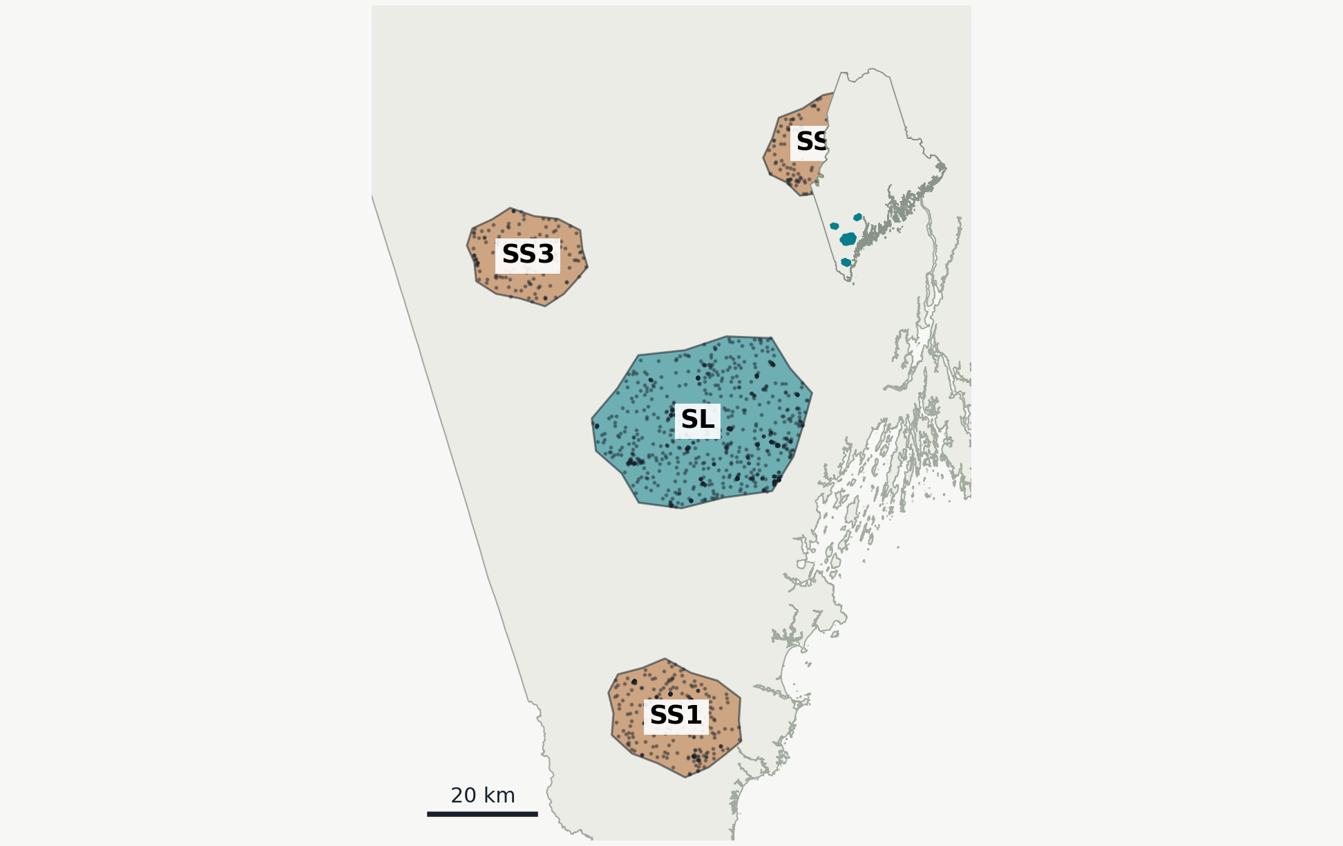
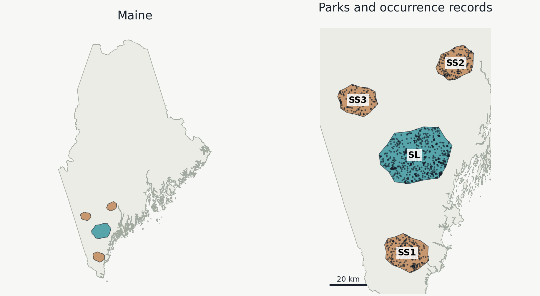
Teal: one large park (1,000 km²). Brown: three small parks (400 + 300 + 300 km²).
This map uses the actual park polygons and occurrence records from Lab10's ME_ImaginaryParks.geojson. The left panel supplies the statewide context; the right panel shows all four parks without an inset covering any park. Only points intersecting the park boundaries are displayed. SL is Alder Basin Preserve; SS1 is Fern Hollow Woods; SS2 is Coldwater Ridge Preserve; SS3 is Spruce Lantern Reserve. The parks are fictional, and the points include both original observations and generated records, including invented species. Each point already has its park ID. The next slide summarizes these park-assigned records as a community matrix, using a small invented example to make the structure readable.
Site-by-species matrix
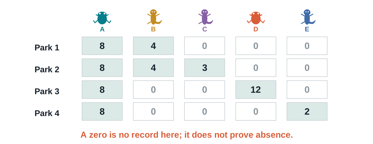
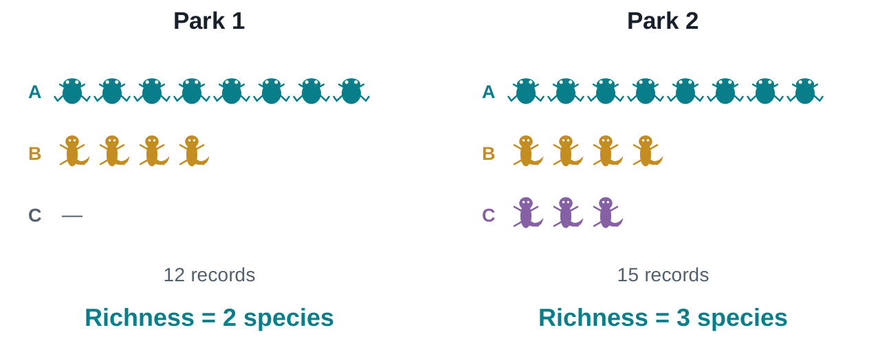
One row per 'community'; one column per species
You can quantify communities using either presence/absence or species abundance, they answer different questions.
Read Park 2 aloud: eight A records, four B records and three C records. Its richness is three, and it has fifteen total records. The same column order must be retained when comparing any rows. Convert positive counts to True for a species-list comparison. A zero can represent true absence, lack of observation or failure to detect. A row of all zeros contains no information for estimating a community's Shannon diversity; do not interpret an empty record set as a confidently species-free park. These are toy counts, not the actual lab matrix. Animal icons are stylized labels; species sharing an icon silhouette are still different species when their letters differ.
Species richness (S)
The most basic measure of community diversity
Richness is simple to interpret, but obviously communities with the same richness can be very different in other meaningful ways.
Each animal icon represents one occurrence record; letters and colors distinguish the invented species. Count the different species, rather than the icons. Additional A records would not increase observed richness, because A is already recorded. One C record in Park 1 would increase its richness to three. Richness ignores how records are divided among recorded species and ignores identities when reduced to a scalar. Two parks can each have richness three while containing entirely different species. Richness can also increase with sampling: more records often discover additional species. We will return to that problem before choosing a reserve strategy.
Entropy / Shannon diversity (H')
How similar are species in their abundances?
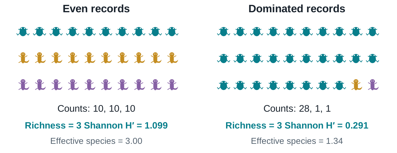
How uncertain would you be about the species of a randomly chosen record?
In the even community, all three species are equally plausible on a random draw. In the dominated community, guessing the dominant species is usually correct. Shannon entropy quantifies that uncertainty. Both richness and balance influence it. In standardized counts of individuals, proportions can represent relative abundance; in this lab they represent relative frequencies of occurrence records. A conspicuous, accessible or heavily reported species can dominate records without dominating the animal community. These values use natural logarithms.
'Effective species' and evenness
Bringing more biological interpretability and comparability across sites
Effective species = exp(H′) Evenness = exp(H′) / S
Counts Richness S exp(H′) Evenness
10, 10, 10 3 3.00 1.00 28, 1, 1 3 1.34 0.45
Shannon diversity is not comparable across sites with different richness. Scaling H' by S gives evenness, which is directly comparable.
The dominated community has the same Shannon diversity as about 1.34 equally frequent species .
The effective count is a comparison with an idealized equally frequent community, not a claim that fractional species were observed. Dividing by richness gives one when all recorded species are equally frequent and a lower value under dominance. This is exp(H)/S, rather than the also-common Pielou measure H/log(S). Keep the name tied to the formula students actually use. Richness is still three in both rows. Empty record sets do not supply an estimable evenness value. Source: Jost explains why transforming entropy into effective numbers gives a more intuitive diversity scale.
Quantifying diversity at different scales; Alpha, Beta, and Gamma Diversity
We want to measure diversity in ways that capture local AND global patterns, and differences among local sites.
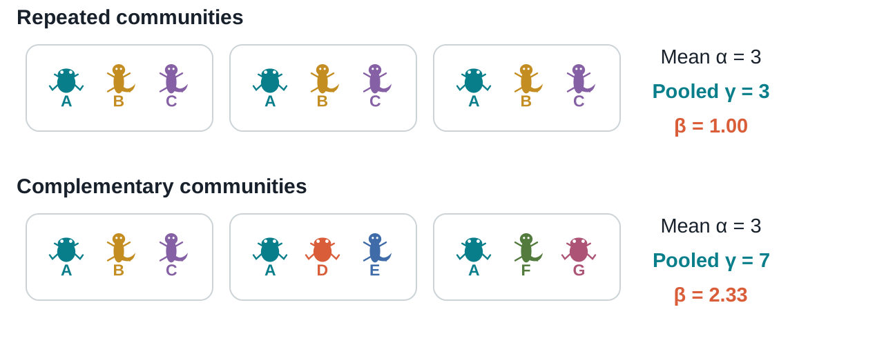
Alpha (α) = local richness. Gamma (γ) = global richness. Beta (β; Average turnover) = γ / mean α.
Larger β values indicate more unique local communities.
Walk through the repeated network first. Adding more copies of ABC does not add species to the pooled list. In the complementary network, A is in all parks while B through G are each in one. The sum of park richnesses is nine in both networks, but gamma is three versus seven. Multiplicative beta is one versus seven thirds. These definitions use richness, with parks weighted equally when averaging alpha. Beta diversity is a family of ideas and measures; state the definition rather than treating every beta index as numerically interchangeable.
Pairwise beta-diversity (presence/absence)
Jaccard Dissimilarity: How much do species lists differ between sites?
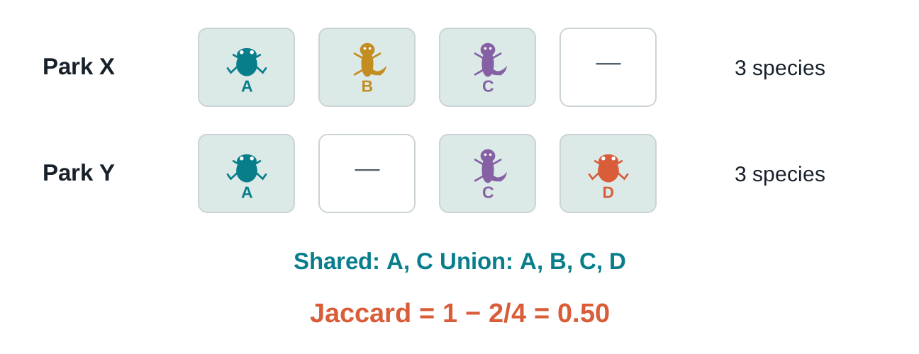
Dissimilarity = 1 − shared / union. Identical lists = 0. No shared species = 1.
Use presence/absence with scipy.spatial.distance.jaccard .
Students can count the shared and union species directly from the figure. A species absent from both lists is excluded from the union and does not make the parks more similar. A rare species recorded once contributes to this presence/absence comparison just as much as a commonly recorded species. Keep the same species-column order for both vectors. SciPy returns dissimilarity rather than similarity. If both parks have no records, a software convention of zero distance supplies no biological evidence of identical communities.
Pairwise beta-diversity (abundance)
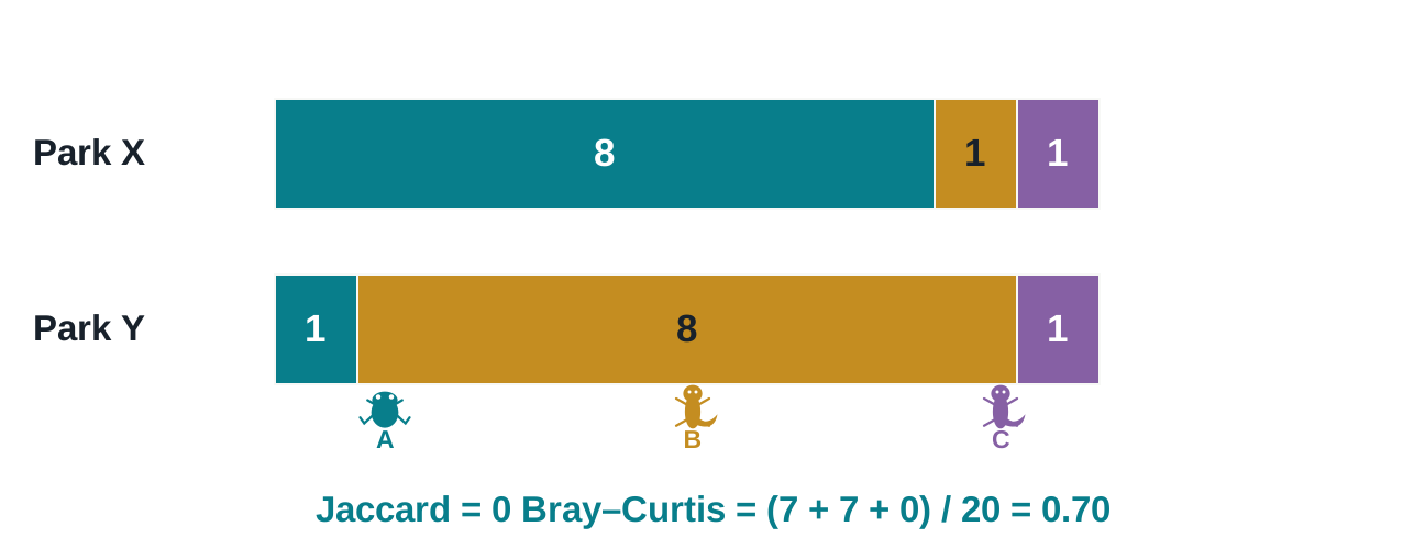
Bray–Curtis Dissimilarity accounts for differences in abundance
Bray–Curtis = Σ |ai − bi | / Σ (ai + bi )
Nonnegative counts; at least one record overall. scipy.spatial.distance.braycurtis .
Both parks contain the same three species, so Jaccard is zero. Species A differs by seven records, B by seven, and C by zero. Dividing fourteen by the twenty total records gives 0.7. For nonnegative vectors with positive combined total, Bray–Curtis lies between zero and one. Zero means identical count vectors; one means no species with positive counts shared. A pair of all-zero vectors has an undefined denominator. The species colors match the icon legend. These invented records illustrate count differences, not inferred animal abundance.
Differential sampling affects observed richness
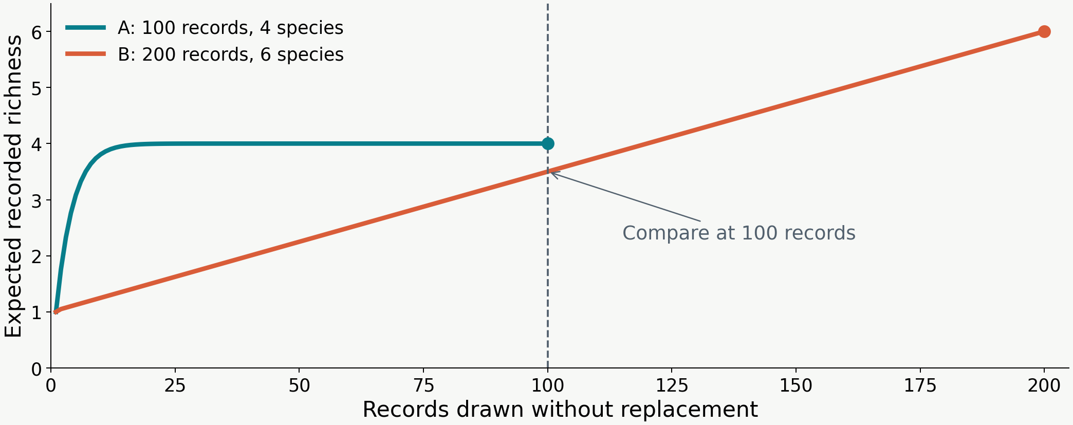
Sample-based rarefaction: Resample to the same number of occurrence data points
Sites with more occurrences may be more species rich because of differential sampling effort. Rarefaction is one way to evaluate sensitivity to this.
These are exact expected richness curves under uniform record draws without replacement, not fitted lab results. At 100 records, A contains its whole sample and therefore all four species. Each singleton in B has a one-half chance of being drawn, while the dominant species is certain to occur, giving one plus five halves, or 3.5. At all 200 records, B has six species. The example shows that dominance and sample size both matter. The lab instead approximates common-size comparisons by repeated draws. Its quantiles summarize draws rather than confidence intervals for true richness. Repeated occurrences need not be independent individuals, so call this record-based rarefaction.
A different conservation objective
Rarity vs Range-restriction
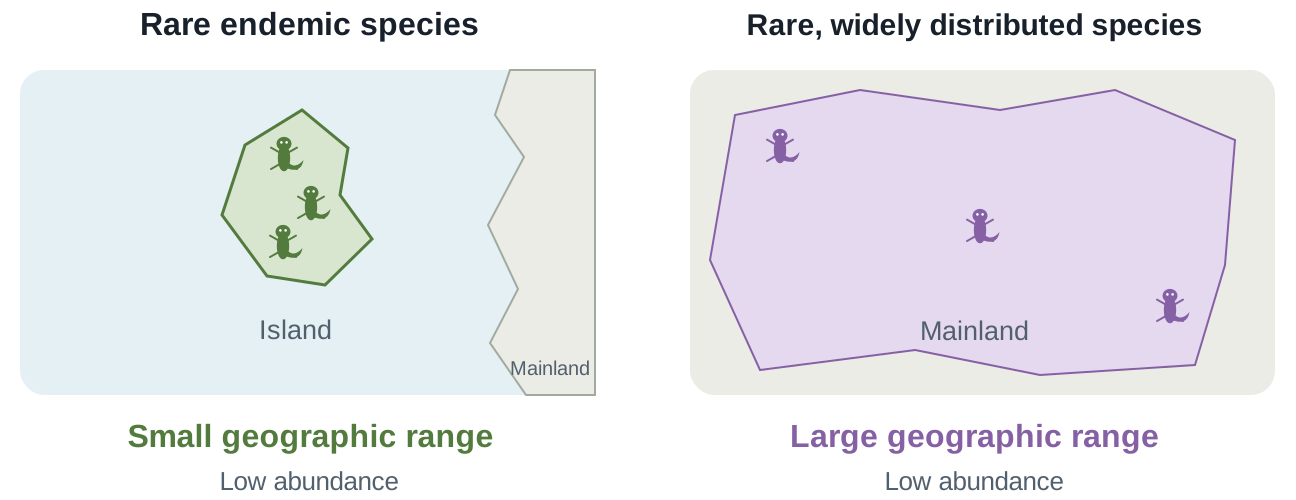
Both have low abundance; only the island species is range-restricted.
Which species would you favor in conservation efforts and why?
Both hypothetical species are uncommon where they occur. Sparse symbols illustrate low abundance on both sides; they are not estimates of total population sizes. The green species' entire range is confined to a small island, so it is both rare and endemic to that island. The purple species is also rare, but occurs at widely separated places across a broad mainland range. Rarity in abundance and restriction in geographic range are different properties. A range-restricted species could also be locally abundant; that combination is not illustrated here. The shaded areas are assumed ranges for these invented examples, not distributions inferred from three observations. In the lab, few occurrence records do not establish low population abundance, and occurrence in only one sampled park does not establish geographic endemism. Daru and colleagues examined how endemism patterns depend on the scope and definition of the analysis. Name the geographic reference explicitly when interpreting range restriction.
Weighted endemism proxy
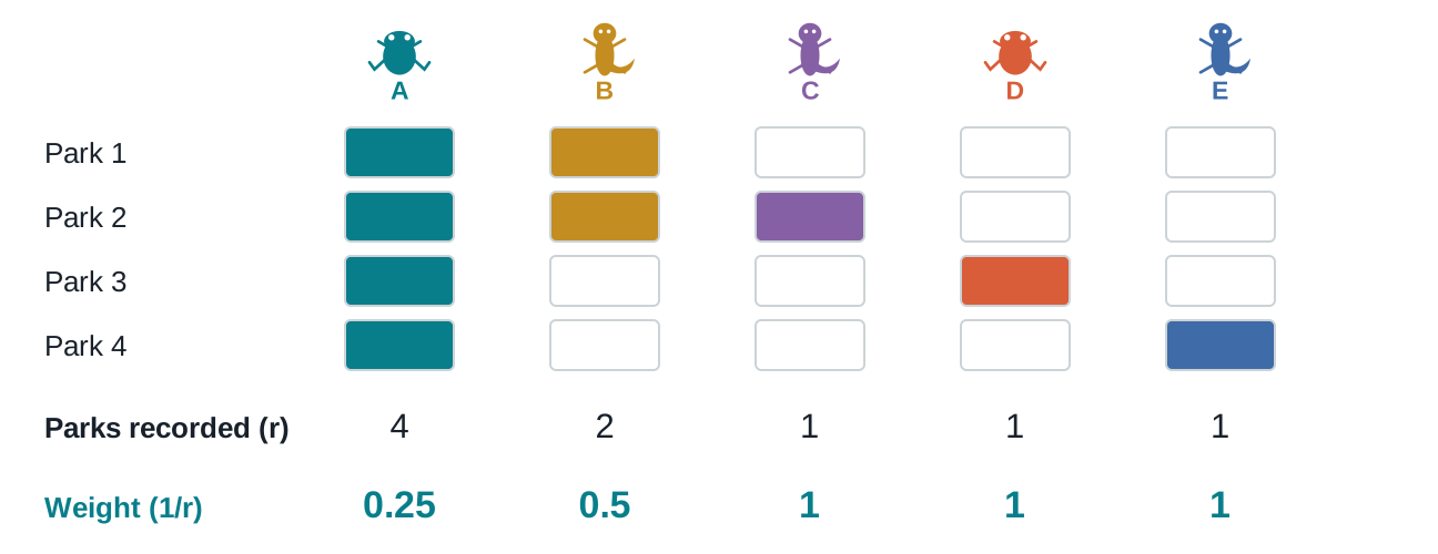
Give more weight to species in fewer parks
For a park: WE = sum of 1/r for its species; r = number of parks recording that species.
Toy park occupancy, not full range size. Range-weighted approach: Crisp et al. (2001) .
Keep the reference set of four parks fixed. Every species in a park contributes something, but a one-park species contributes four times as much as a four-park species. A's abundance of eight in each park does not enter this weight. WE is a sum, so it can increase by adding species even if those species are widespread. Published geographic WE commonly weights by occupied geographic units across a broader range. Our park-based version is a proxy; units differ in area and the available occurrences do not constitute complete range maps. The formula teaches the inverse-occupancy logic without claiming calibrated regional endemism.
Weighted versus corrected weighted endemism
A sum and an average can rank parks differently
Toy park Species WE CWE = WE / S
Park 2 A, B, C 0.25 + 0.50 + 1 = 1.75 0.58 Park 3 A, D 0.25 + 1 = 1.25 0.625
WE: total contribution of richness and restriction.
CWE: mean restriction weight of the species recorded.
Would adding a widespread species necessarily improve CWE?
No. Adding a species with a weight below the current average increases WE while decreasing CWE. Park 2 has the larger sum, but Park 3 has a larger average restriction weight. Neither is a universally superior conservation score. CWE is not an independent estimate of range rarity and does not automatically remove sampling bias. The worked values use the same matrix as the preceding slides. Crisp et al. 2001 introduced the correction to help distinguish endemism patterns from species richness; keep that distinction tied to the conservation objective.
Rarity is not a single property
Few records and narrow ranges are different
Toy species Total records Parks recorded Record-rare?
A 32 4 No C 3 3 Yes D 12 1 No E 2 1 Yes
Species 'C' is rare but widespread. Species 'D' is abundand but localized. Species 'E' is both rare and range-restricted.
C and D are both sample-exclusive, but only C is record-rare. E also meets both conditions. A hypothetical species with one record in every park would be record-rare while having the maximum park occupancy, demonstrating the opposite combination. The threshold of five is a teaching choice, not a biological boundary or conservation designation. A low count might reflect low abundance, poor detectability, little reporting or the simulation's allocation. Some invented species have only a few points by design. Ask students how changing the threshold to ten would affect the species counted and whether that should change their conservation recommendation.
Return to the conservation question
Build a recommendation from several lines of evidence
Evidence Question for the recommendation
Pooled richness and complementarity Which species would each strategy represent? Shannon and evenness How much does record dominance affect the comparison? Jaccard and Bray–Curtis Do lists, counts and relative frequencies tell the same story? Common-size resampling Does the ranking persist at equal record numbers? Restriction and record rarity Which otherwise missed species might matter?
Explain disagreements among metrics; they often reveal different biological priorities.
Avoid combining all indices into an unexplained score. A strong recommendation states its objective, identifies species gained or missed, reports numerical evidence and explains uncertainty. If one strategy has greater gamma while another has higher CWE, that is not a mathematical contradiction. It is a choice between total representation and average restriction under the chosen proxy. A focal-species protection objective could justify a different choice again. The records cannot tell us which outcome the community or society should value most.
Further reading
Conservation and diversity concepts
Sources support the conceptual explanations; numerical examples in the lecture are our own teaching examples, not extracted study results. SLOSS has a much larger literature than the short historical motivation here. The goal is to prepare an explicit representation comparison while retaining the biological limits of that comparison.