Lab 11 · November 13, 2026
Spatial Analysis of Community Composition
How can we quantify change in community composition as a function of geography and environment?
From aggregated occurrence records to spatial community turnover, how do we get there?
BIO597 Spatial Analysis of Biodiversity
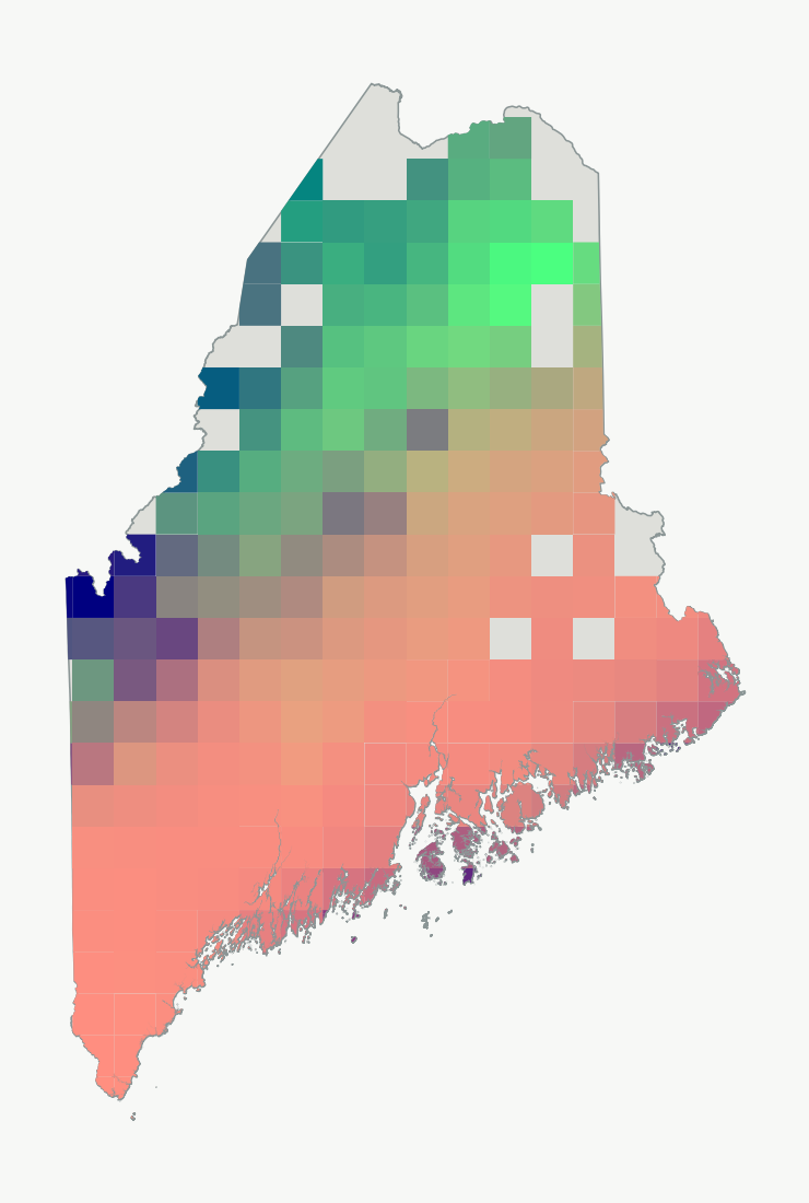
Amphibian community similarity as a function of environment (similar colors indicate more similar communities)
How do communities change across the landscape?
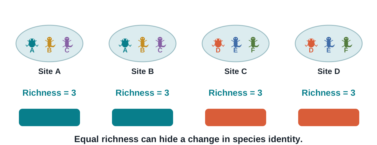
Well, how do we quantify community change? Richness is one dimension. Community composition another.
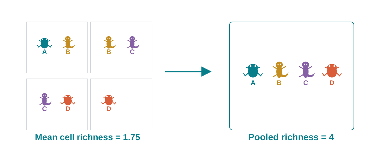
A richness map can remain constant while community composition changes completely.
From observations to communities
How do we delineate communities?
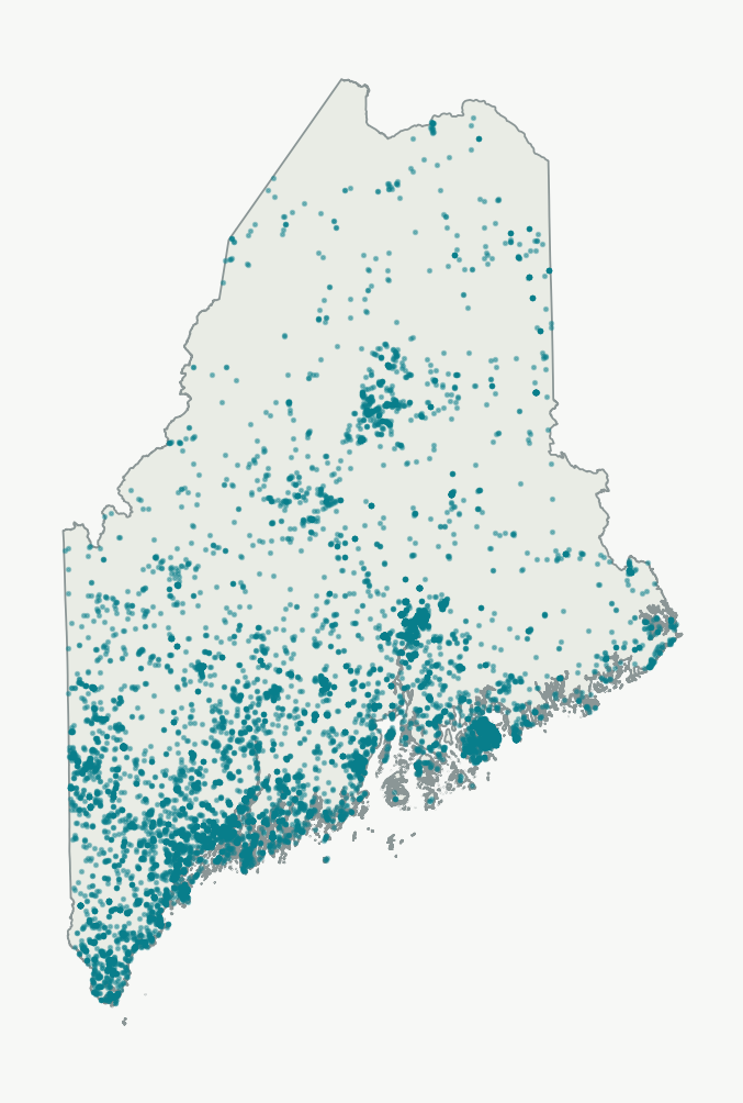
The points locate observations; we still need to define the sites we compare.
Original Maine data · amphibian occurrence records used in Lab11.
If we have spatially continuous samples, how do we determine 'communities'?
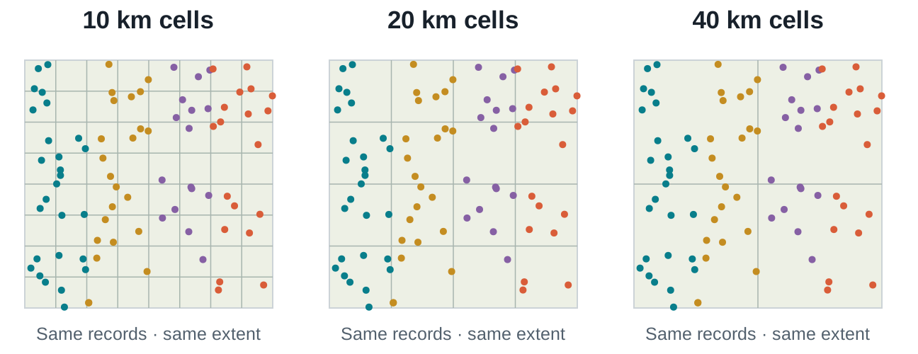
The same points can form different communities
A simple way is to partition the landscape into grid cells with a given grain (grid cell size)
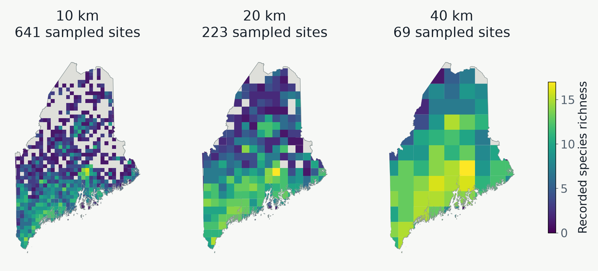
The size of the gridcell will determine community composition.
What aggregation does
A larger cell pool more species
Increasing grain may (or may not) increase species richness of a grid cell.
This may (or may not) have consequences for downstream analysis, and this is one of the things we will explore in the lab today.
Species richness as a function of grid cell size for ME amphibians
How do richness patterns change as a function of spatial grain?
Larger cells contain more pooled species.
Are these patterns largely concordant or discordant as grain size increases?
Quantifying community difference
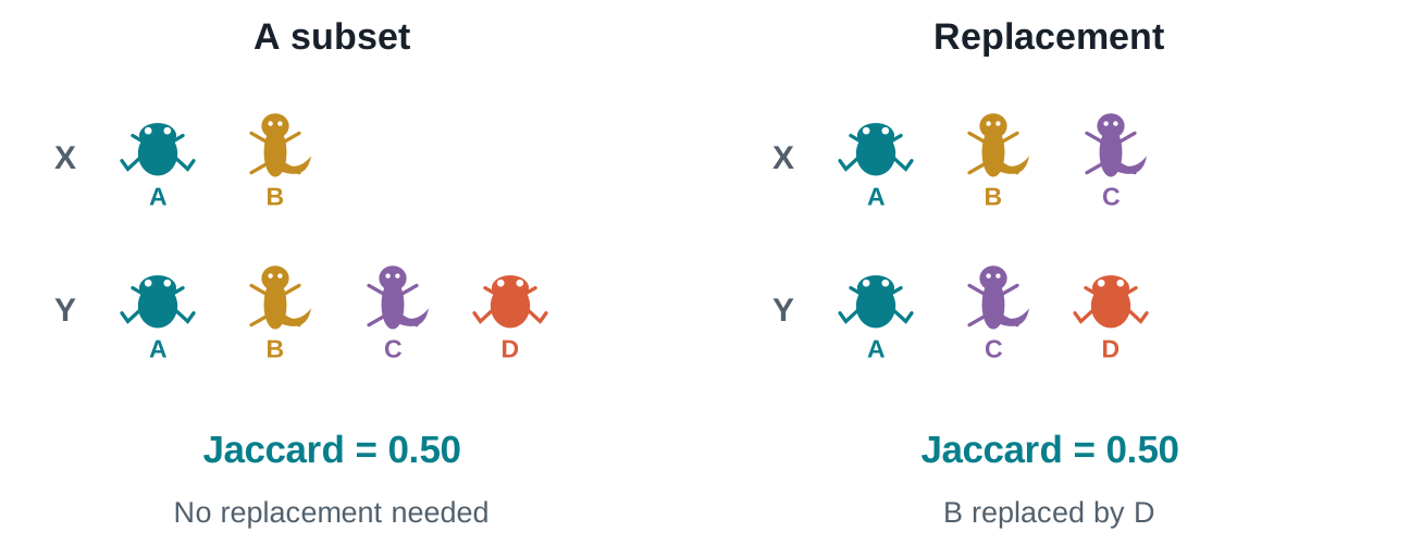
Two patterns can determine community difference
Jaccard dissimilarity (difference in community composition) can include replacement and nestedness.
Nestedness means one community is a subset of another
Pairwise dissimilarity for all communities
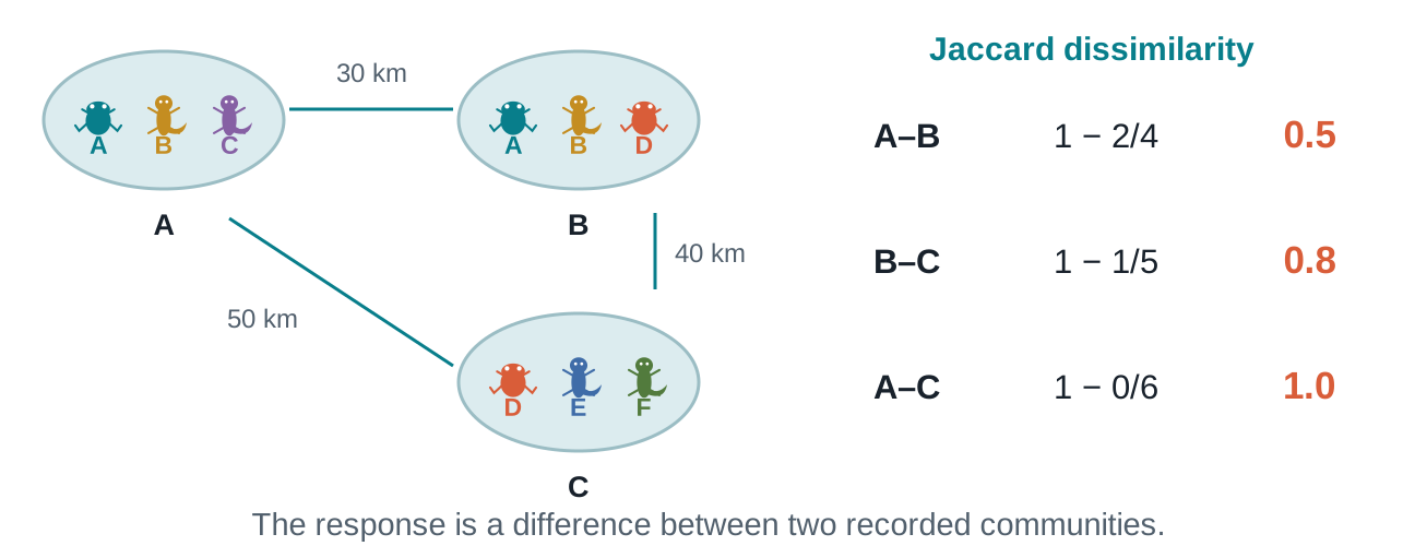
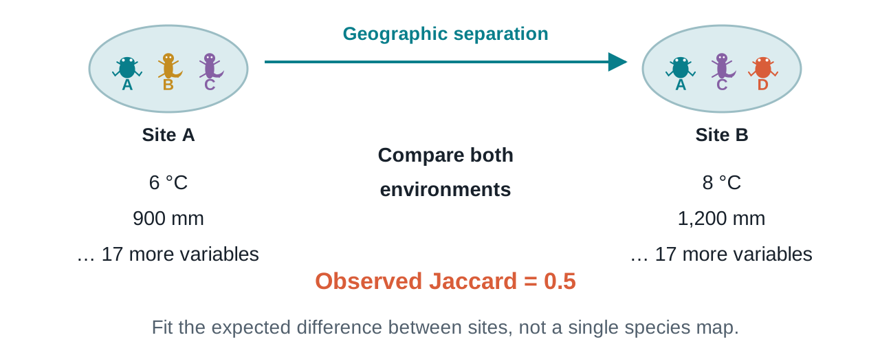
Each comparison needs two species lists
Keep site order aligned when pairing species differences with geographic distances.
Worked example · Jaccard = 1 − shared / union; schematic distances, not to scale.
Distance decay of similarity
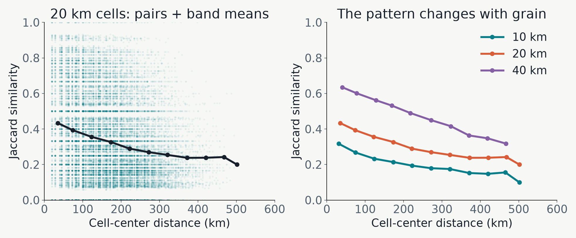
Do distant sites share fewer recorded species?
Distance decay summarizes a pattern. Its strength and shape can change with grain.
Original Maine data · points = pairs; lines = means in 50 km distance bands.
Community change over the landscape
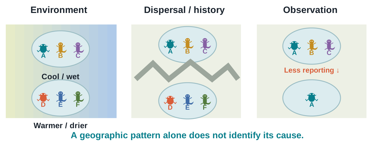
Several processes can produce distance decay
Environment, dispersal, history, and observation can act together.
Neighborhood similarity
Which recorded communities differ nearby?
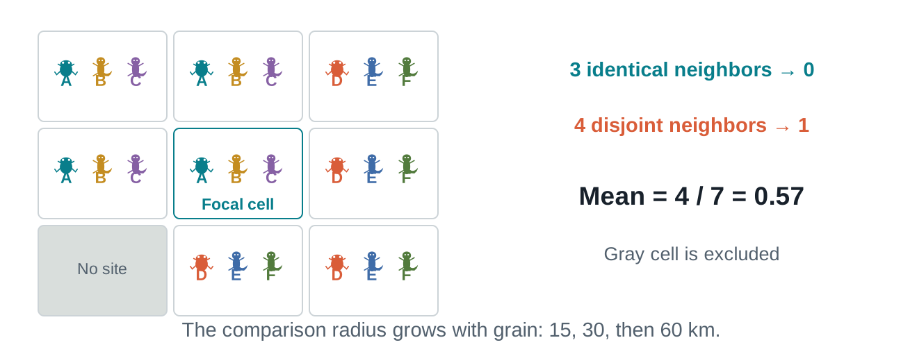
Mean neighbor Jaccard describes local compositional difference.
Worked example · same-radius comparisons are made within each grain.
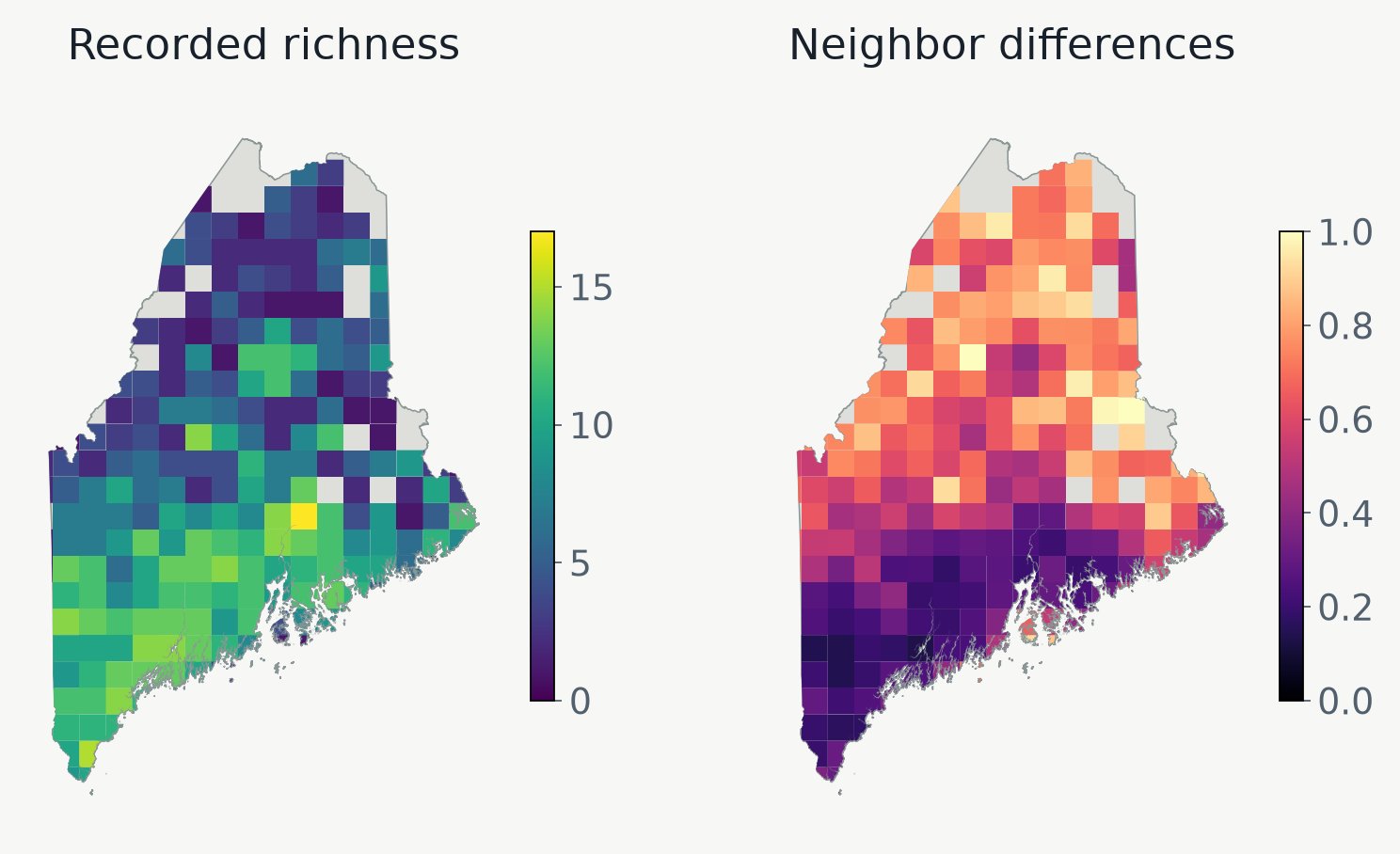
Richness and difference answer different questions
A rich site need not be the most distinctive
Use the species lists and record totals to interpret a high local difference.
Original Maine data · gray indicates no mapped value, not zero difference.
Add environmental context
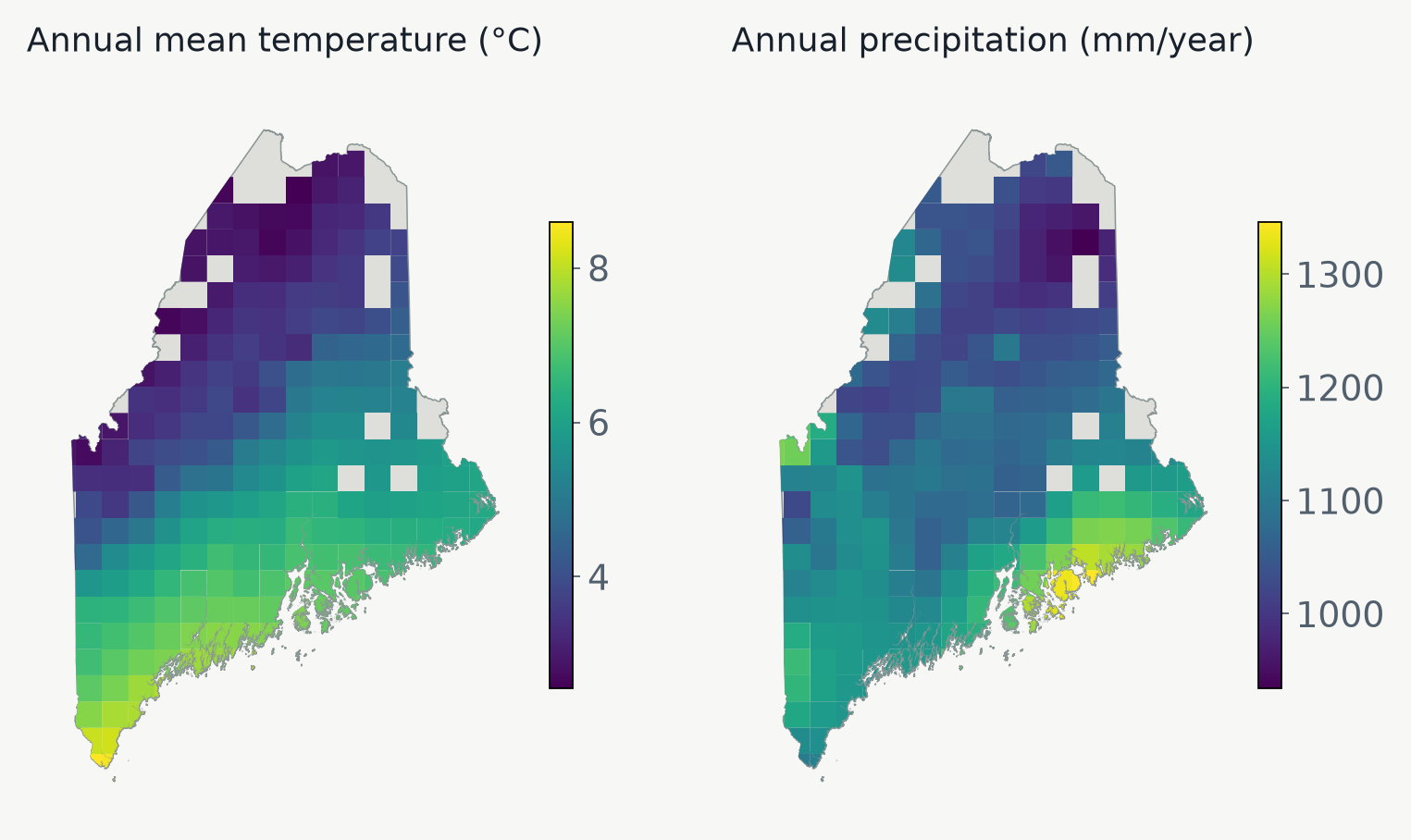
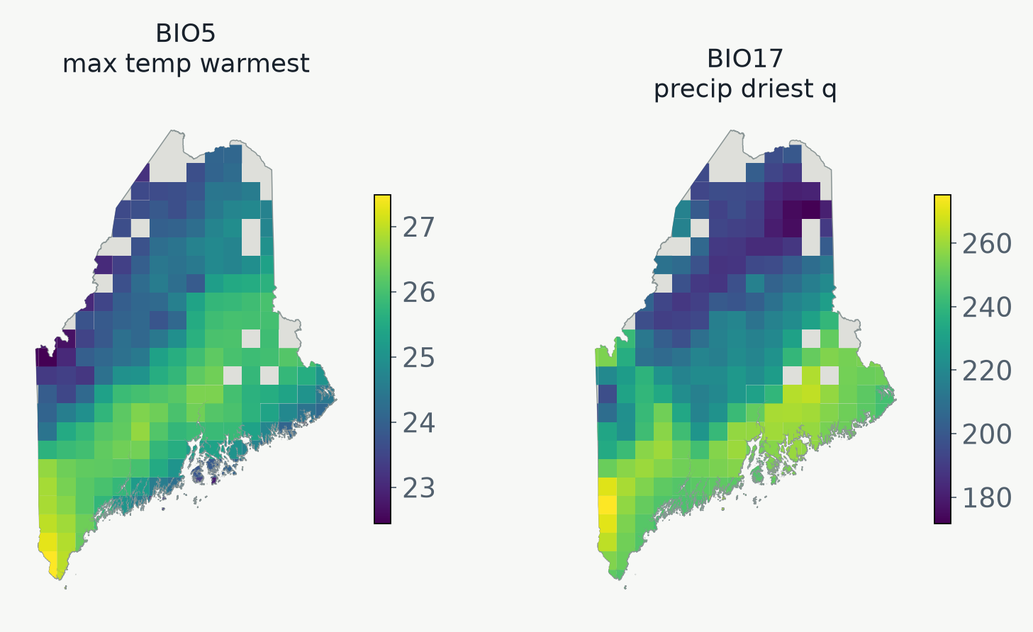
A site has an environmental setting
All 19 bioclimatic variables enter GDM; these two maps orient us to the landscape.
Original Maine data · WorldClim variable definitions.
The main nonlinear intuition
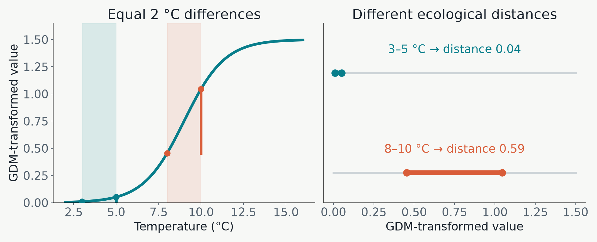
Equal climate steps need not mean equal change
GDM stretches parts of a climate gradient where communities change more.
Illustrated transformation · this curve is not a fitted lab result.
Environmental correlates of community turnover
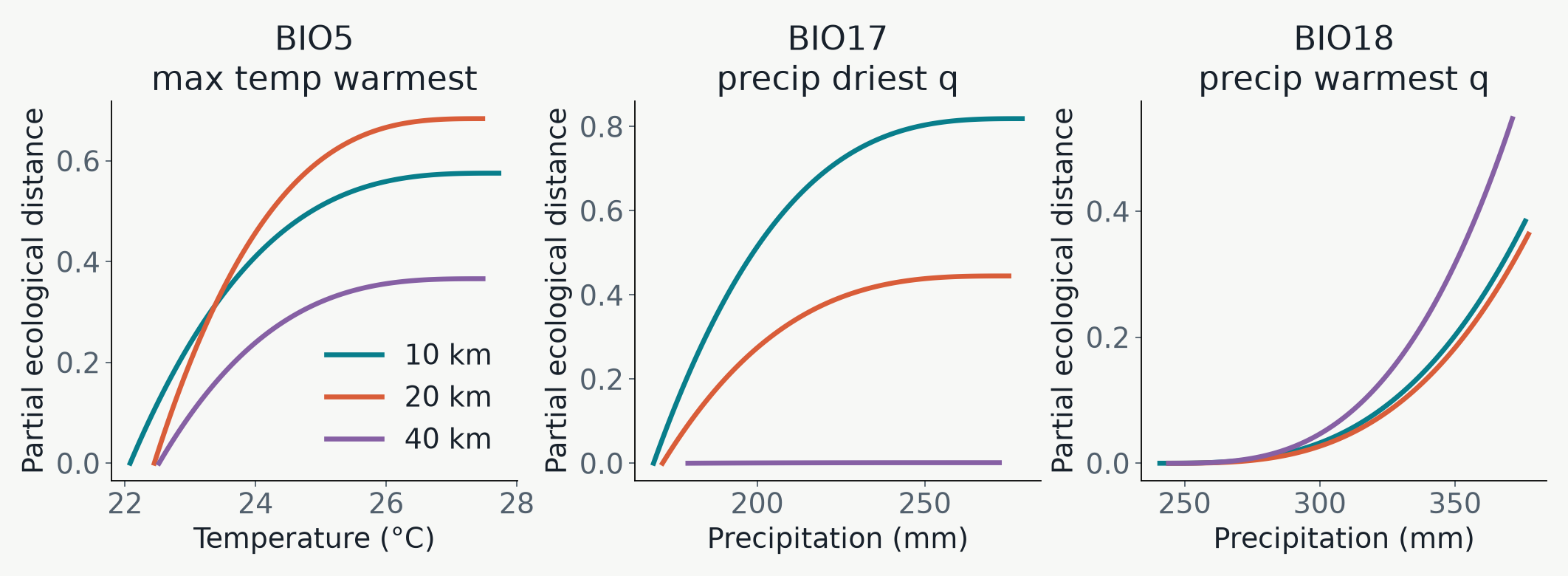
Steep segments identify intervals of modeled change
Read the slope and climate interval, then compare grains.
Original Maine data · all curves come from models using all 19 predictors.
Projecting estimated community turnover across the landscape
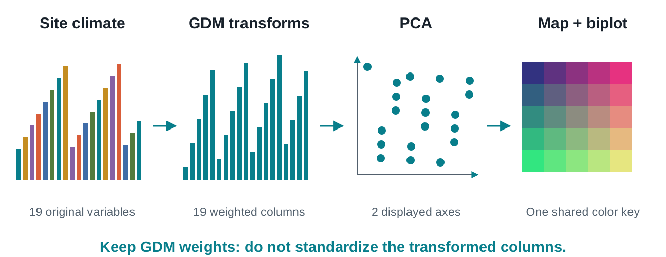
Summarize the transformed environments
Transform first, then use PCA to display the major axes of expected compositional variation.
Method: PCA · implementation: gdmbayes.
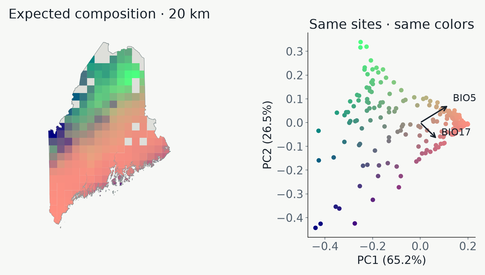
One color key in two spaces
Nearby colors summarize similar expected composition
PC1 + PC2 retain 91.7% of the GDM-transformed variation.
Original Maine data · first two PCs; geographic-distance effects are excluded from the site colors.
Connect the ordination to environmental biology
Which gradients align with the displayed change?
Two longest arrows: BIO5 and BIO17.
Original Maine data · select by length in the PC1–PC2 plane; display only two arrows.
Choose the map for the biological question
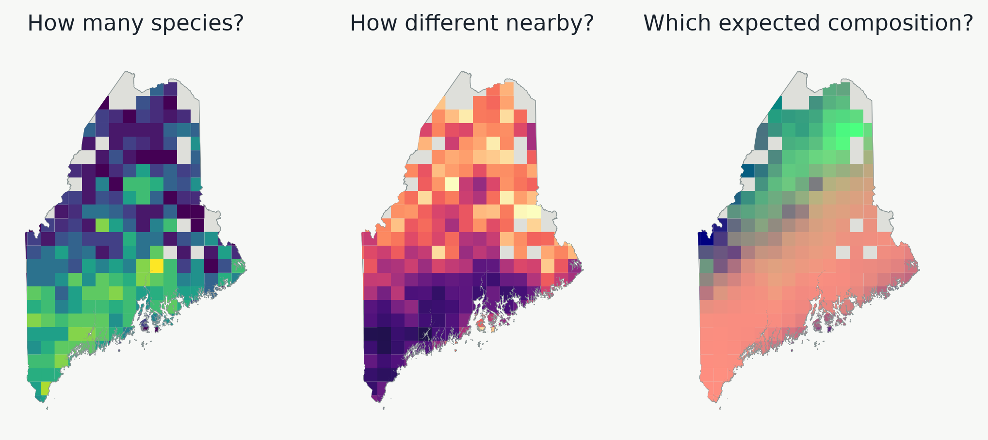
Three maps, three different kinds of evidence
Which map would help locate a richness hotspot, a local contrast, or an environmental transition?
Original Maine data · each panel answers a different question; colors are not interchangeable.
Readings and figure provenance
Methods behind the pictures