Week 12 · BIO597 Spatial Analysis of Biodiversity

Spatial trait-based ecology

Where do richness and functional diversity disagree? What processes can this tell us about?
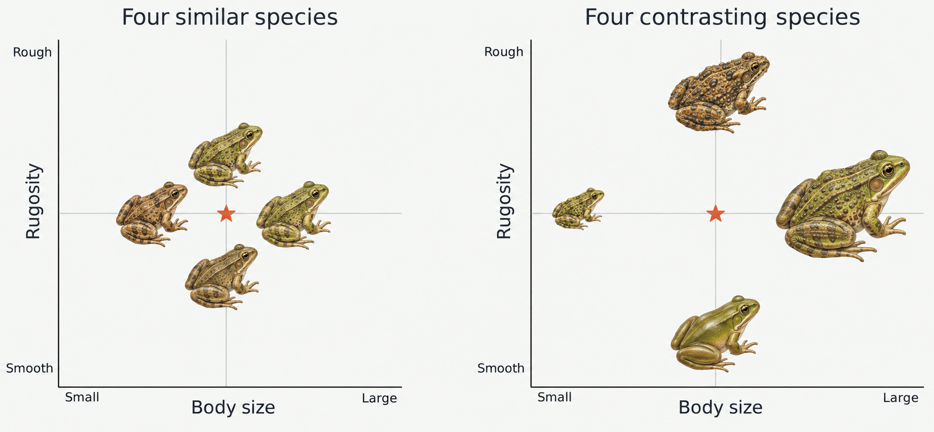
Two hypothetical four-species communities shown with frog illustrations on body size and rugosity axes. One contains similarly sized, moderately textured frogs; the other includes small, large, smooth, and rough-skinned frogs.

Both communities have four species, but one has much higher functional diversity (trait variation).

How does environment and geography influence life history at the species and community level?
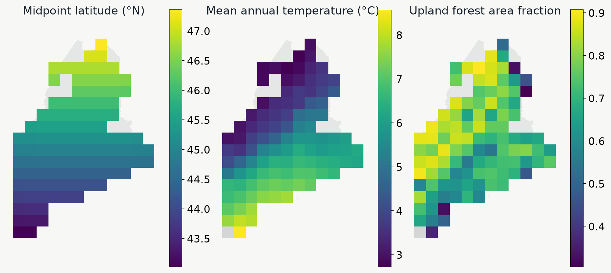
Three Maine maps show a north–south latitude gradient, spatial temperature variation, and the proportion of mapped area covered by upland forest.

Which life-history strategies or traits occur along gradients of latitude, climate, and habitat?

Bergmann's rule: Larger bodied species found in colder environments (true for endotherms).

Compile amphibian trait data

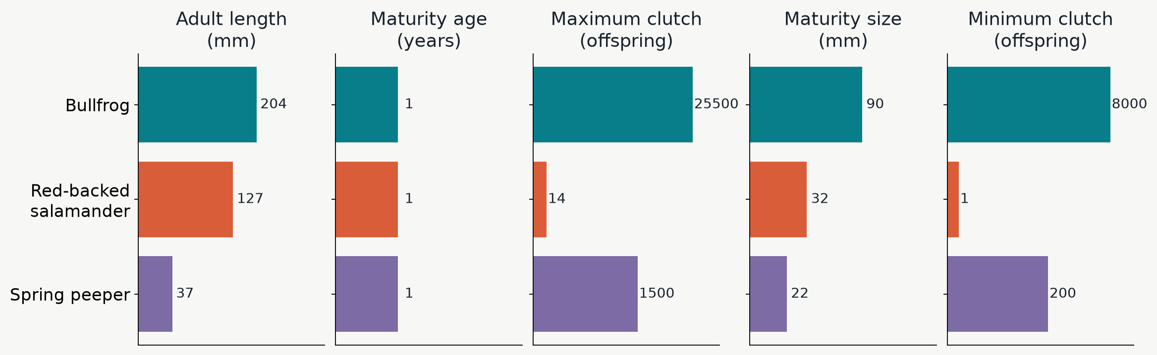
Five traits describe size, maturity, and reproduction
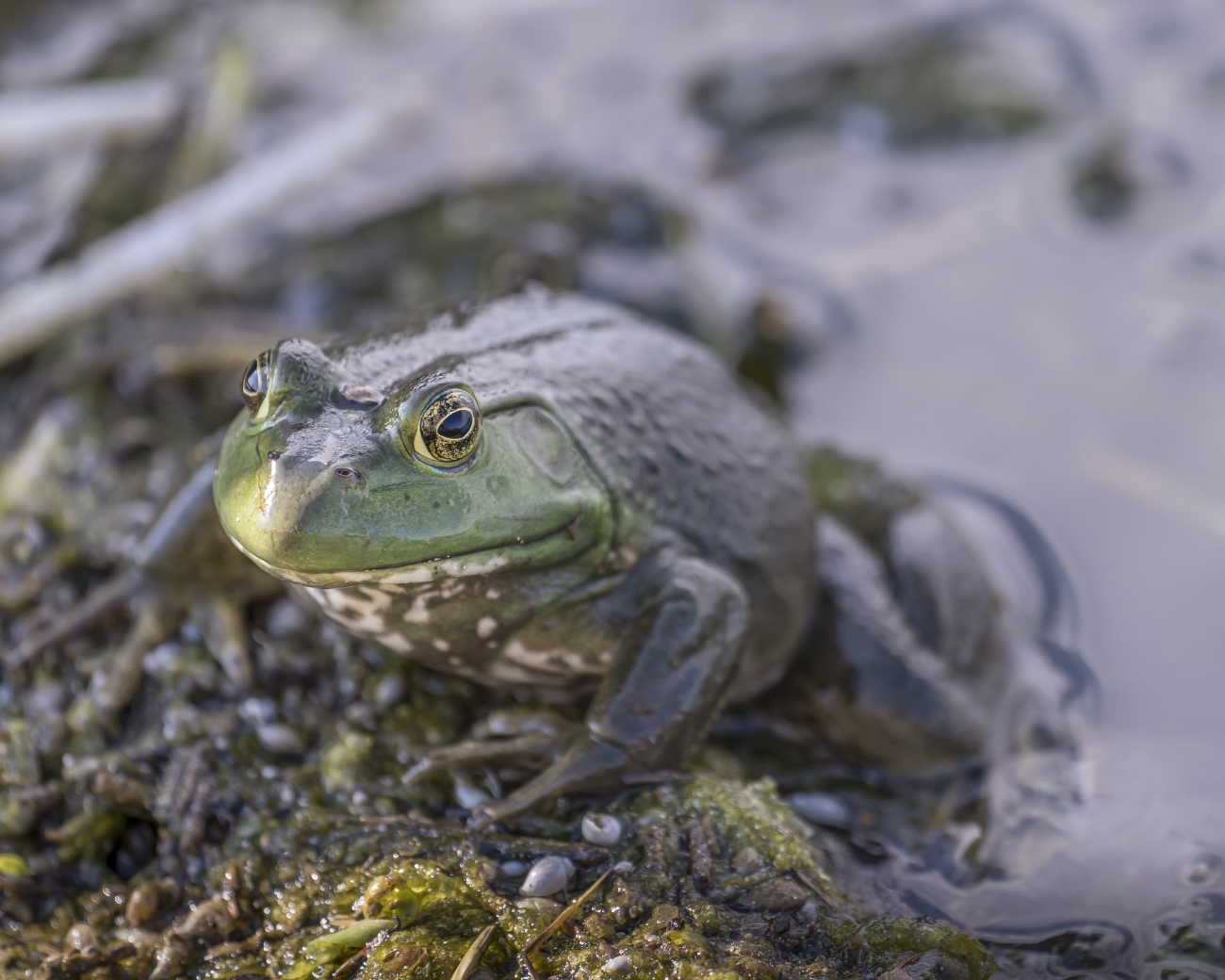
American bullfrog, Lithobates catesbeianus
American bullfrog
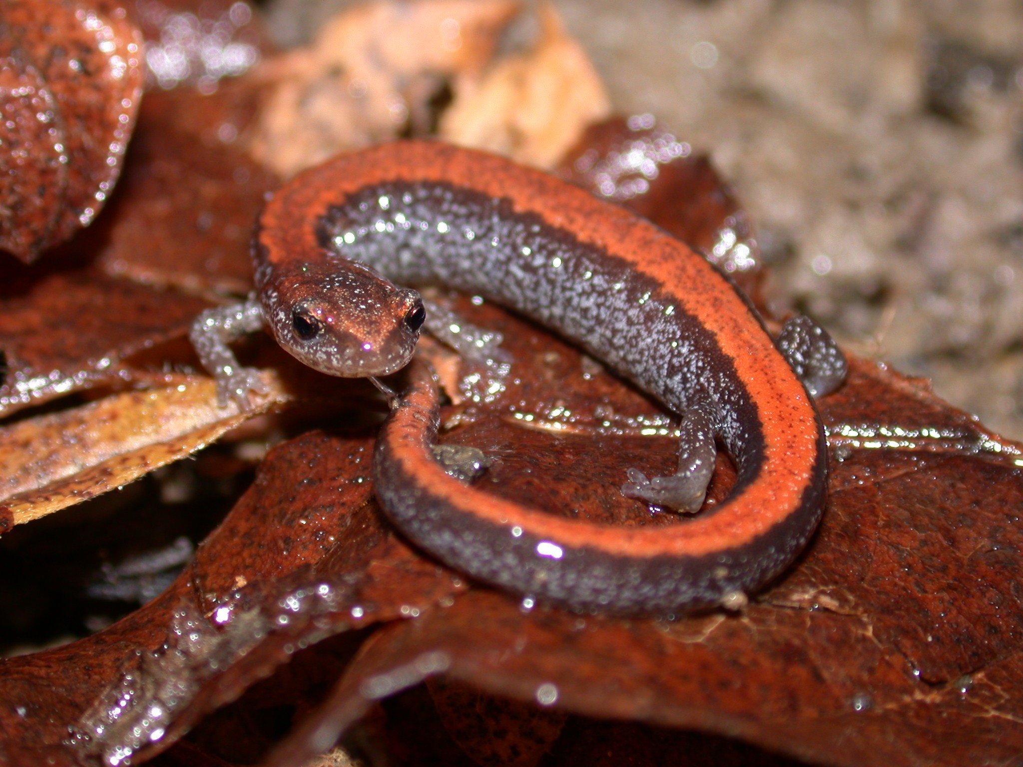
Red-backed salamander, Plethodon cinereus
Red-backed salamander
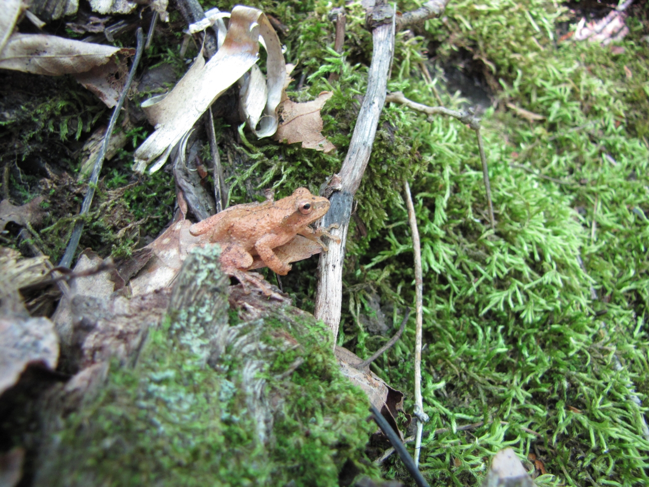
Spring peeper, Pseudacris crucifer
Spring peeper
Five panels show maximum adult length, minimum maturity age, maximum clutch size, minimum maturity size, and minimum clutch size for three Maine species.

The trait table gives each species a life-history profile.

Scaling and standardizing for comparability

Make proportional changes comparable

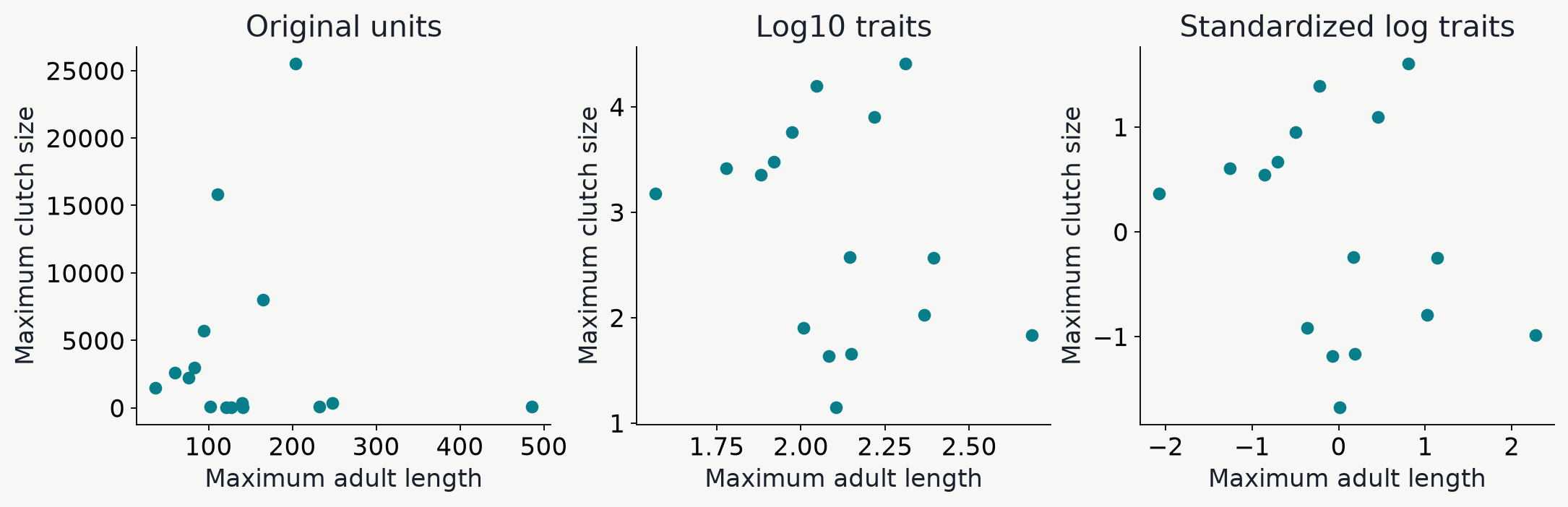
Three Maine scatterplots show body length versus maximum clutch size in original units, log10 units, and standardized log units.

Log10 makes proportional differences comparable; standardization gives each trait equal variance.

Here each point is a species.

The first spatial question

Where do community mean traits change?
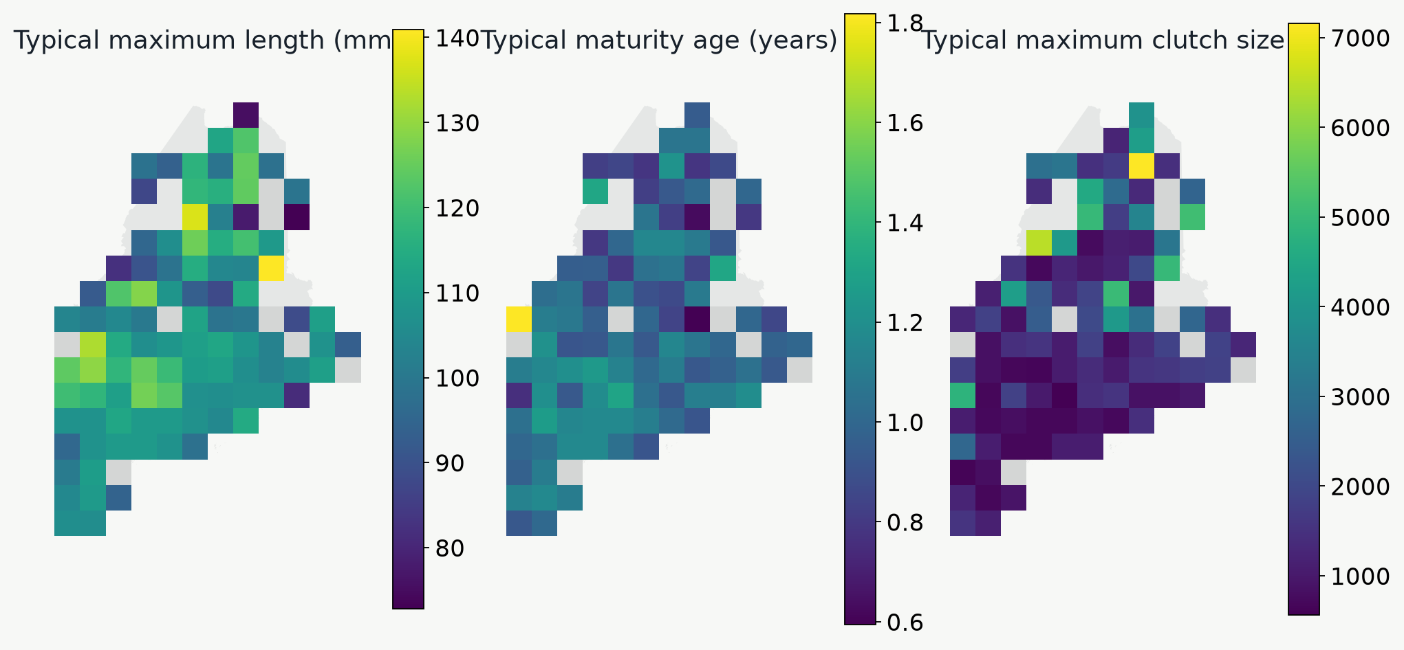
Maine maps show geometric means of maximum body length, minimum maturity age, and maximum clutch size for cells with adequate trait coverage.

Do colder or more disturbed places contain species with different body sizes, maturity ages, or clutch sizes?

Correlating environmental predictors with mean community traits

Which environmental gradients accompany shifts in mean traits?
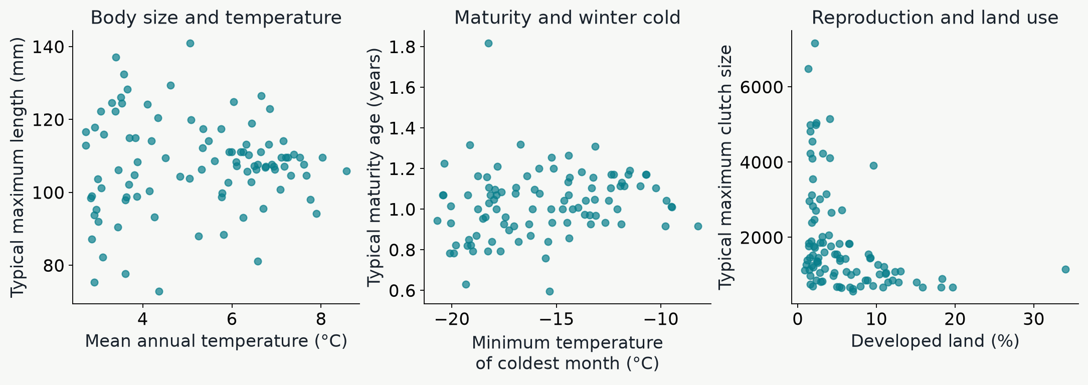
Three empirical Maine scatterplots compare typical maximum body length with annual temperature, maturity age with coldest-month temperature, and maximum clutch size with the percentage of developed land.

Do any of these relationships look meaningful to you? How would you interpret these figures?

Here each point is a community average.

Summarizing trait variation w/in communities (Functional diversity)

Functional dispersion (FDis) is the mean distance to the multivariate trait centroid

Two hypothetical four-species communities shown with frog illustrations on body size and rugosity axes. One contains similarly sized, moderately textured frogs; the other includes small, large, smooth, and rough-skinned frogs.

In this cartoon the centroids of these two communities are identical

Species in the community on the right occupy a wider spread of the measured trait space, so it will have a larger FDis value

A worked example for ME amphibians

These two real communities have very different FDis values
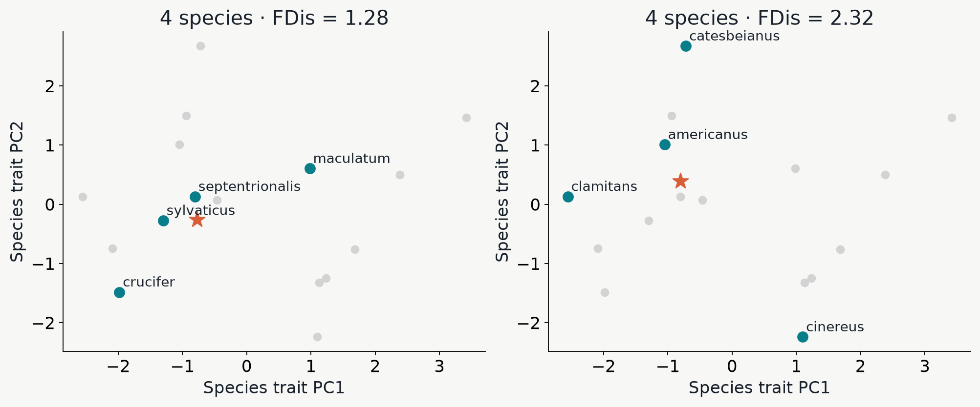
Two Maine communities with four species are highlighted on the same regional species PCA; their full-space functional dispersion differs.

The red star indicates the centroid in multivariate trait-space for the given community

How similar are communities in trait-space?

PCA applied to species+traits versus communities+trait means
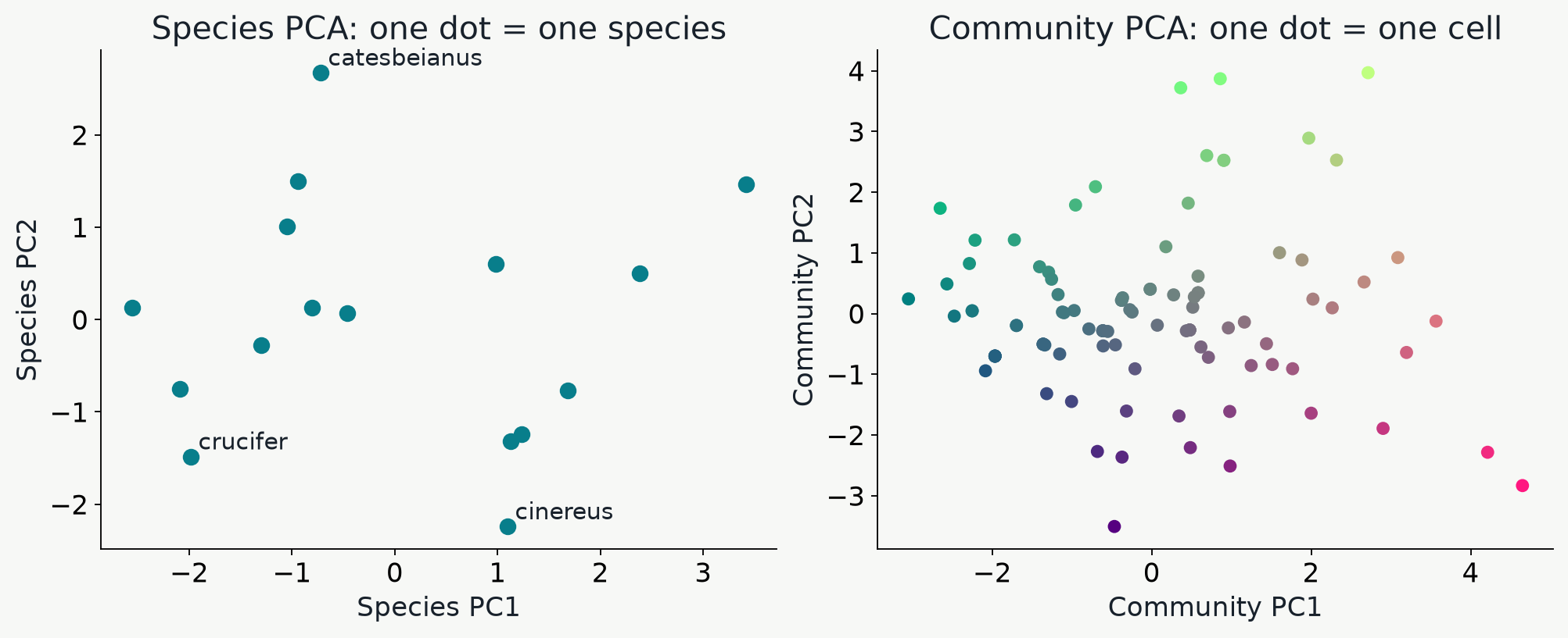
A Maine species PCA with one dot per species is shown beside a separate PCA of five community mean traits with one dot per retained cell.

Nearby species have similar trait profiles. Nearby communities contain species with similar average traits.

How do biotic and abiotic interactions shape community trait distributions?

Filtering favors similarity; competition can favor divergence
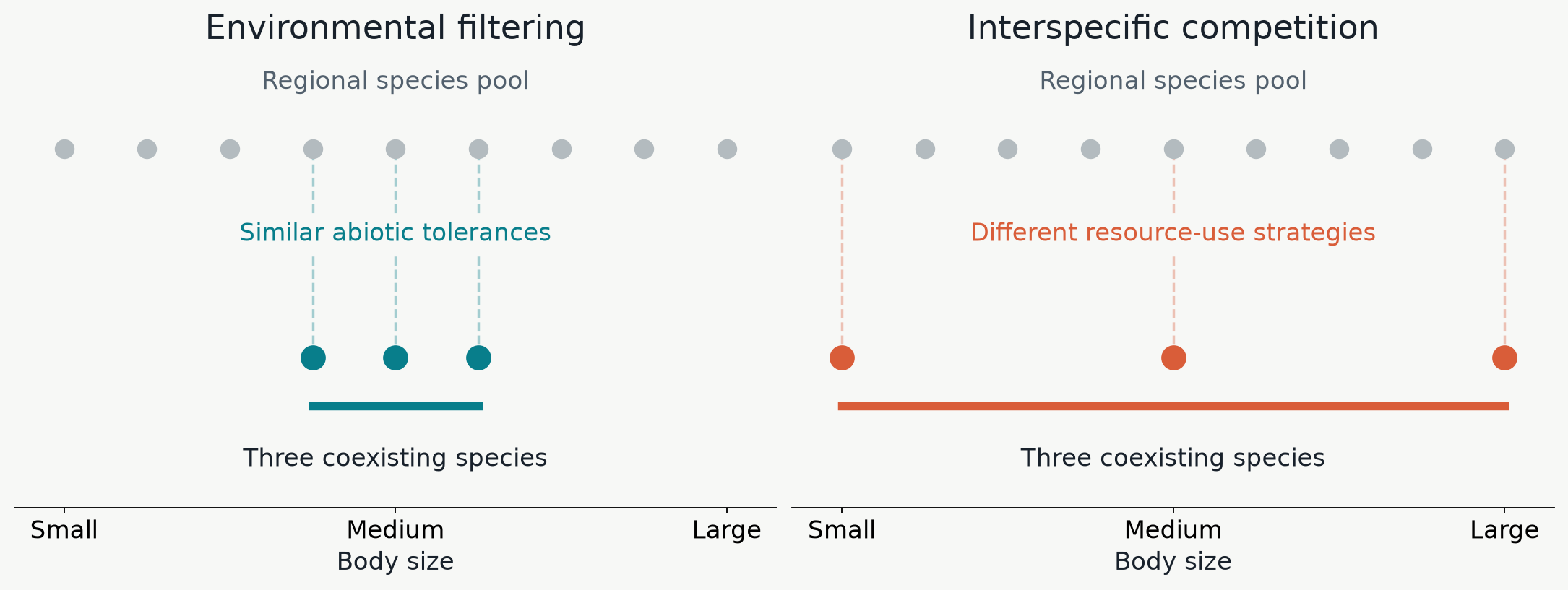
Two hypothetical assembly scenarios start with the same nine-species regional body-size distribution. Environmental filtering retains three similarly sized species, while interspecific competition favors three widely spaced body-size strategies. Both local communities have three species.

Abiotic constraints can favor similar species; resource competition can favor dissimilar coexisting species.

Testing the ecological hypotheses with trait randomization

Within each site: Shuffle rows of the trait dataframe; recalculate FDis; repeat 1000x
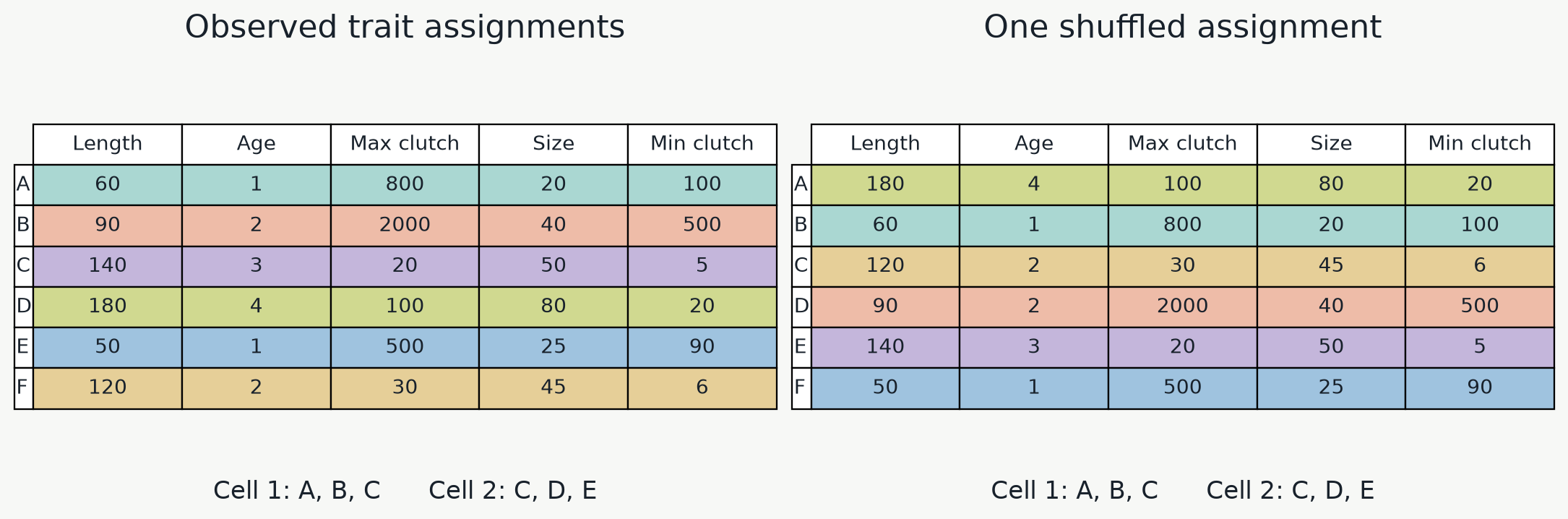
Two tables show a joint permutation of five-trait rows among fixed species A through F. The same cell species lists remain below both tables.

The distribution of FDis values can be used get a p-value for the observed FDis

Observed versus null distribution of FDis values

Is the observed functional dispersion significantly different from randomized FDis?
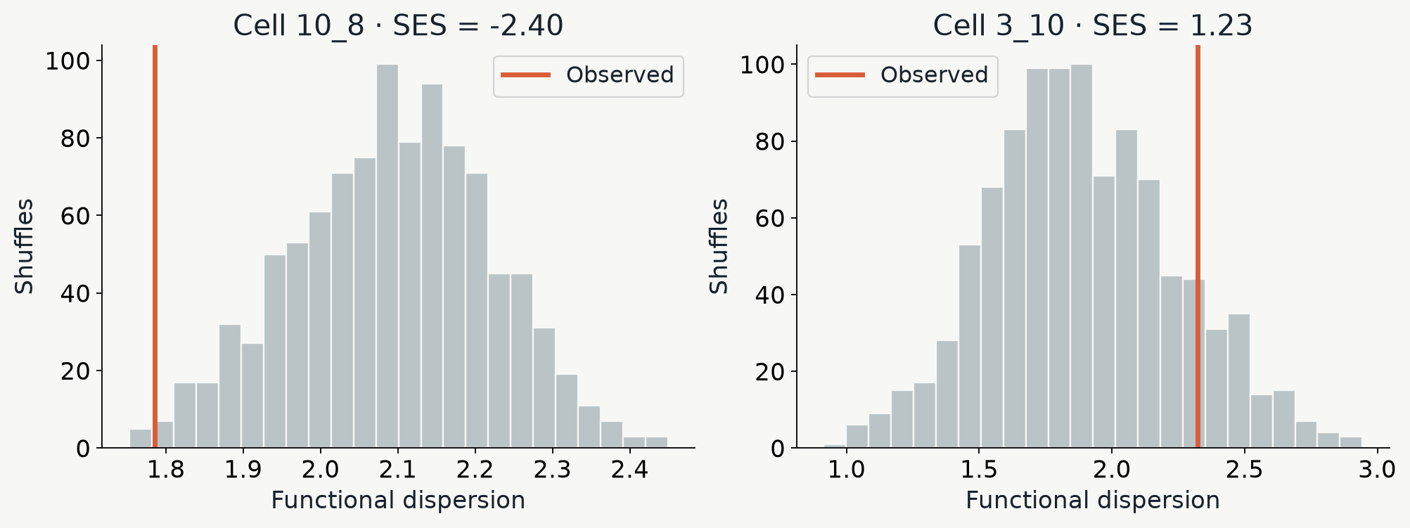
Two Maine histograms show randomized functional dispersion and the observed values for cells with contrasting standardized departures.

The standardized effect size (SES) is (observed FDis - null mean) / null SD.

Negative values indicate clustering; positive values indicate greater spread than expected.

Looking at spatial patterns of FDis

Where is functional dispersion significantly smaller relative to the regional pool?
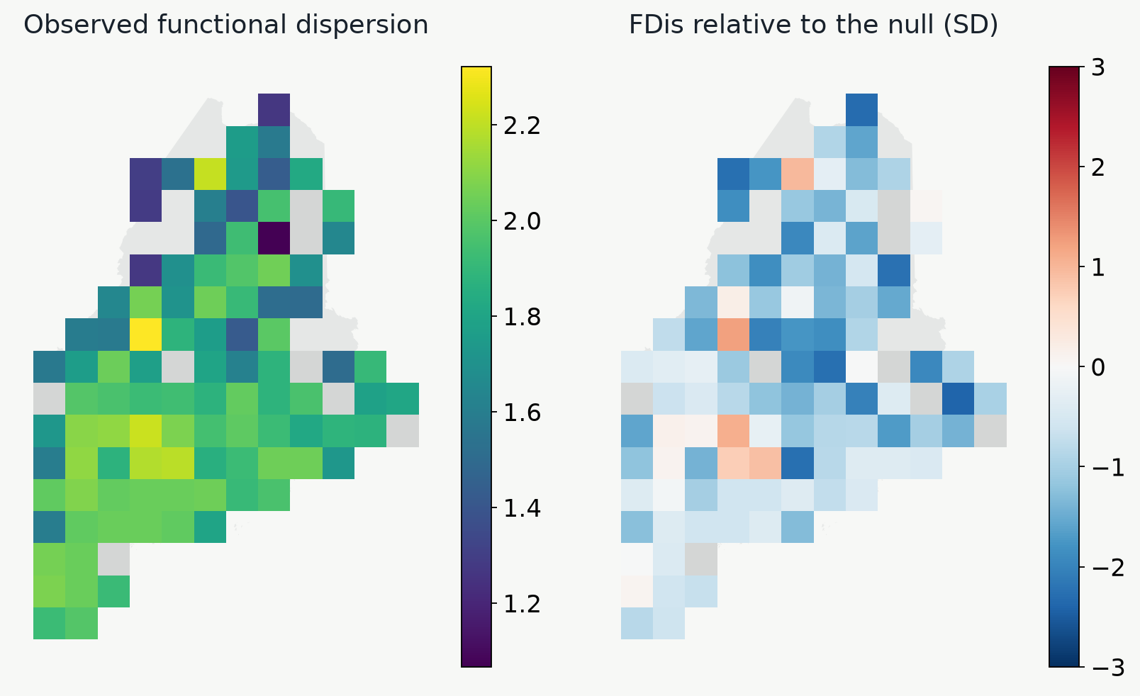
Maine maps compare raw functional dispersion with the standardized effect size relative to the trait-shuffling null model.

One might hypothesize that colder climate would impose an environmental filter

How would you interpret the spatial pattern of FDis here?

Connecting FDis to environmental predictors

How does trait dispersion vary with environment?
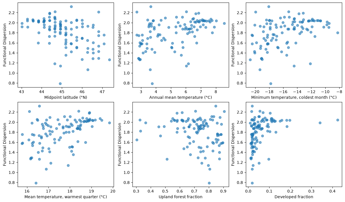
Six scatterplots from Lab12 Step 4 show community functional dispersion against midpoint latitude, annual mean temperature, coldest-month minimum temperature, warmest-quarter mean temperature, upland forest fraction, and developed fraction. All correlations use Pearson r.

Each panel relates community trait dispersion (FDis) to environment, latitude, and habitat type

Connecting traits to environment

Which gradients track community life-history strategies?
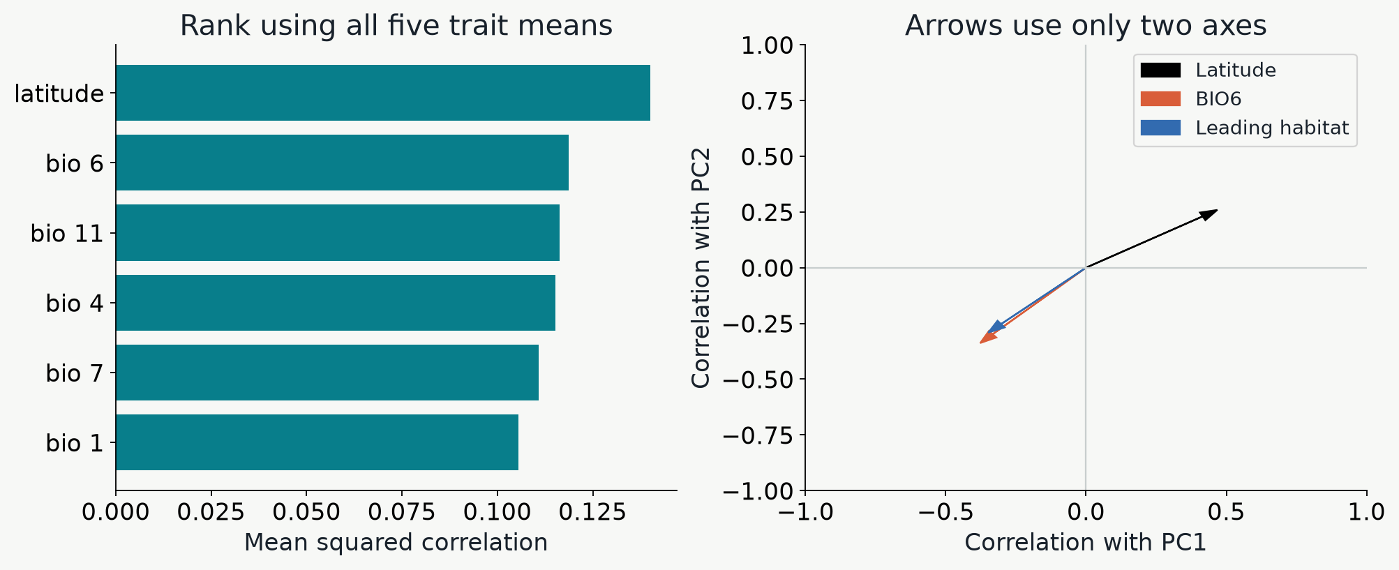
A bar chart ranks Maine predictors by mean squared correlation across five trait means, beside arrows based only on correlations with PC1 and PC2.

Use the ranking to identify associated gradients and the arrows to see how trait combinations change along them.

Putting it all together

How does environment drive similarity in community trait composition?
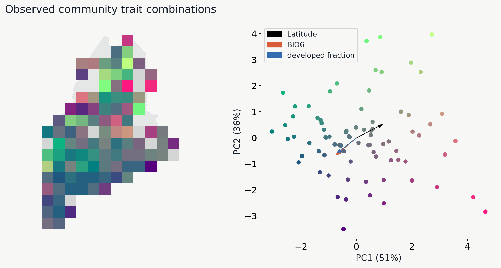
A Maine grid map colored by community PCA scores is paired with the same colored cells in PCA space and three predictor arrows.

Similar map colors identify communities with similar combinations of mean life-history traits.