BIO597 Spatial Analysis of Biodiversity Fall 2026
Simple python data structures - List & Dictionary
Lists
Lists are one of the fundamental data structures in python. They are optimized for performance and simplicity. They are similar to vectors/lists in R, while requiring much less typing for most operations.
# A list of strings
fruits = ["apple", "banana", "cherry"]

# A list of mixed data types
mixed_list = [42, "hello", True, 3.14]

# An empty list
empty_list = []
%whos
Variable     Type    Data/Info
------------------------------
empty_list   list    n=0
fruits       list    n=3
mixed_list   list    n=4
# List indexing

# Python lists are 0-indexed. The beginning of the list is element 0 and
# the end of the list is element n-1 (where n is the number of items in the list).

fruits = ["apple", "banana", "cherry"]

print(fruits[0])   # Output: apple
print(fruits[2])   # Output: cherry
print(fruits[-1])  # Output: cherry (counting from the end of the list with negative numbers
apple
cherry
cherry
# Useful list operations

numbers = [1, 99, 2, 3, 4]

print(len(numbers))     # len() is 'length': 5
print(sorted(numbers))  # Sort the list: [1, 2, 3, 4, 99]
print(numbers[::-1])    # Black magic to reverse the order of items: [4, 3, 2, 99, 1]
numbers.append(42)      # [1, 99, 2, 3, 4, 42]

print(fruits + numbers)        # join 2 lists together (concatenate): ['apple', 'banana', 'cherry', 1, 99, 2, 3, 4, 42]
5
[1, 2, 3, 4, 99]
[4, 3, 2, 99, 1]
['apple', 'banana', 'cherry', 1, 99, 2, 3, 4, 42]
# Looping over list items

for n in numbers:
    print(n)
1
99
2
3
4
42
Dictionaries - Native key/value pairs
A Python dictionary (or dict) is a built-in data structure used to store data in key-value pairs. Unlike lists, where elements are accessed by their position (index), dictionary values are accessed using a unique key. Dictionaries are ordered (they remember the insertion order), mutable (you can change them), and do not allow duplicate keys.
The closest R equivalent is a named list:
user <- list(username = "ecology_student", followers = 1500)

# Using double square brackets
print(user[["username"]])  # Output: "coder123"
## The python dictionary equivalent of this is:

user = {"username":"ecology_student",
        "followers":1500,
       }

## Access dictionary value associated with a given key
print(user["username"])

## Get a list of keys from a dictionary
print(user.keys())
ecology_student
dict_keys(['username', 'followers'])
## Looping over dictionary items

for key in user:
    # Print the key and the value of the key in the dictionary
    print(key, user[key])
username ecology_student
followers 1500
Introduction to pygbif and GBIF occurrence data
Goals for today
This notebook introduces the basic workflow for using Python to fetch biodiversity occurrence records from GBIF.
By the end of this lab you should be able to:
- search for a species name in the GBIF taxonomic backbone
- find the GBIF taxon key for a species
- count available occurrence records
- download a small number of occurrence records
- convert those records into a
GeoDataFrame - plot the records on an interactive map
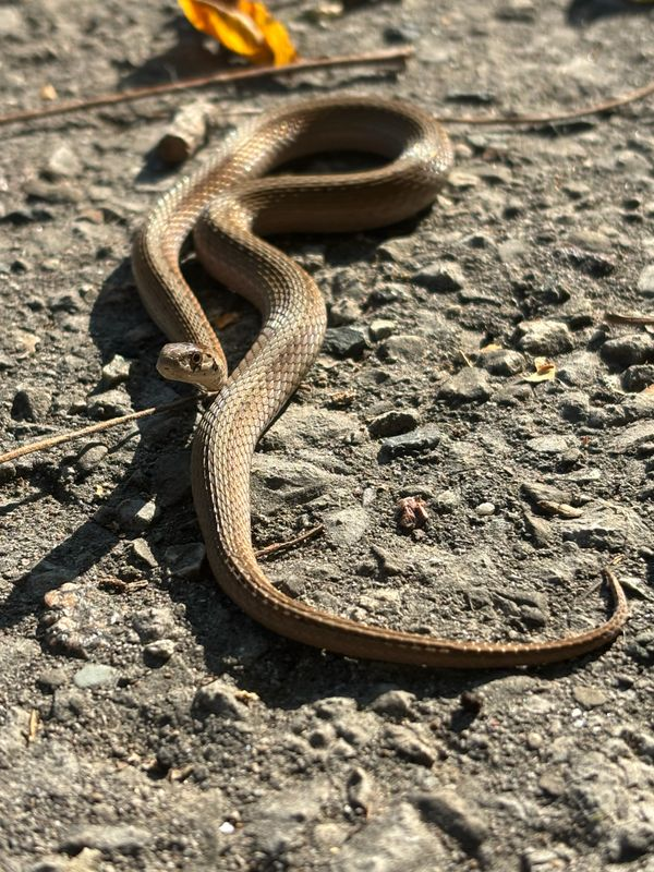
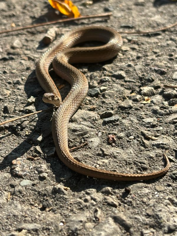
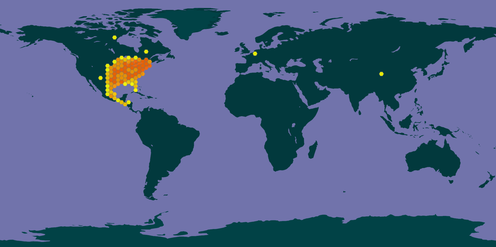
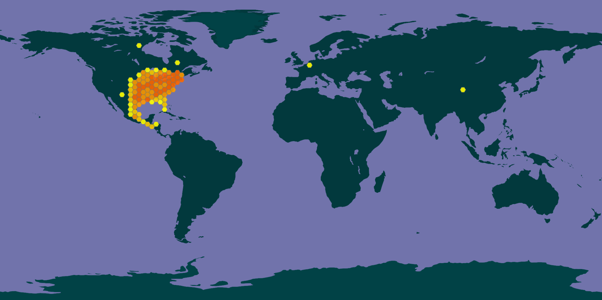
We will use DeKay's brownsnake, Storeria dekayi, as the example species.
What is GBIF?
GBIF is the Global Biodiversity Information Facility. It is one of the most important online repositories for biodiversity datay. It brings together biodiversity occurrence records from museums, research collections, community science projects, and other sources.
An occurrence record is usually a record that a species was observed or collected at a particular place and time. Occurrence records are usually georeferenced (i.e. they include decimal latitude and longitude), but not always, and sometimes the latlongs are wrong, so data cleaning is important.
Today we will use pygbif(pygbif homepage), a Python package that talks to the GBIF API from inside a notebook.
Prerequisites
If pygbif is not already installed, open a terminal and run:
pip install pygbif
This lab also uses geopandas and pandas, which we used in Lab 01.
1. Import packages
We will import two parts of pygbif:
species, for searching taxonomic namesoccurrences, for searching occurrence records
We will also use pandas for tables and geopandas for spatial data.
from pygbif import species
from pygbif import occurrences as occ

import pandas as pd
import geopandas as gpd
2. Search for a species name
Before downloading occurrence records, we need GBIF's taxon key for the species (called speciesKey). The taxon key is a unique numeric identifier used by GBIF. As you might guess, there are taxon keys across different levels of the taxonomic hierarchy (there are genusKey, familyKey, and so on, up to kingdomKey).
name_suggest() does a simple search for names that match the text we provide (it's not very smart). This is useful when you are checking spelling or trying to see what GBIF knows about a name.
The funciton may return more than one result, so the output is a list where the zero-th element is the most relevant. We will inspect it first, then pull out the speciesKey in the next cell.
name_results = species.name_suggest(q="Langaha")

# name_suggest() returns a list of dictionaries in descending order of relevance.

# Look at the zero-th element of name_results, which is itself a dictionary
first_name_result = name_results[0]

first_name_result
{'key': 8286831,
 'nameKey': 18932547,
 'kingdom': 'Animalia',
 'phylum': 'Chordata',
 'family': 'Pseudoxyrhophiidae',
 'genus': 'Langaha',
 'kingdomKey': 1,
 'phylumKey': 44,
 'classKey': 11592253,
 'familyKey': 10874056,
 'genusKey': 8286831,
 'parent': 'Pseudoxyrhophiidae',
 'parentKey': 10874056,
 'nubKey': 8286831,
 'scientificName': 'Langaha Bonaterre, 1790',
 'canonicalName': 'Langaha',
 'rank': 'GENUS',
 'status': 'ACCEPTED',
 'synonym': False,
 'higherClassificationMap': {'1': 'Animalia',
  '44': 'Chordata',
  '11592253': 'Squamata',
  '10874056': 'Pseudoxyrhophiidae'},
 'class': 'Squamata'}
## Try printing a list of the keys in first_name_result
3. Get a more sophisticated match if you aren't sure of the scientific name
pygbif species module has another function called name_lookup(). This service uses fuzzy lookup so that you can put in partial names and you should get back those things that match
dekayi_lookups = species.name_lookup(q="Storeria d")

print(f"I got {len(dekayi_lookups)} matches for this search.")
I got 6 matches for this search.
4. Save the taxon key
The value called usageKey is the GBIF taxon key we will use for occurrence searches.
dekayi_key = name_results[0]["genusKey"]
dekayi_key
8286831
5. Count matching occurrence records
Before downloading records, it is useful to ask GBIF how many records match our search.
Here we count records for Storeria dekayi that are georeferenced. Georeferenced records have coordinates, which means we can map them.
dekayi_count = occ.count(
    taxonKey=dekayi_key,
    isGeoreferenced=True,
)

dekayi_count
49081
6. Fetch up to 100 occurrence records
Now we will fetch occurrence records using occ.search().
For this lab, keep the search small. We will request a maximum of 100 records with limit=100.
The GBIF API may have many more matching records than this. Limiting the request keeps the notebook fast and makes the output easier to inspect.
dekayi_records = occ.search(
    taxonKey=dekayi_key,
    #hasCoordinate=False,
    #hasGeospatialIssue=False,
    #year="1900,2000",
    limit=300,
)

print(len(dekayi_records['results']))

# Search records are dictionaries (and they can be large), so look first
# at the available keys. Look at the keys and see if you can guess what
# the associated value of each key means.
dekayi_records.keys()
281


dict_keys(['offset', 'limit', 'endOfRecords', 'count', 'results', 'facets'])
## In this cell try accessing each key in the dekayi_records dictionary
## to verify what the content is and to see if your intuition about it is correct
7. Look at one occurrence record
The search result is a dictionary. The actual occurrence records are stored under the results key.
Look at the first record before turning all of the records into a table.
dekayi_records["results"][0]
{'key': 675715501,
 'datasetKey': 'b6015b60-6f96-43a9-88e5-2f41854e8f07',
 'publishingOrgKey': '2b8e48b0-812d-11de-86fe-b8a03c50a862',
 'networkKeys': ['68e8e67a-43e6-44a3-8817-dc0e6b70f973',
  '99d66b6c-9087-452f-a9d4-f15f2c2d0e7e'],
 'installationKey': 'a957a663-2f17-415f-b1c8-5cf6398df8ed',
 'hostingOrganizationKey': '2053a639-84c3-4be5-b8bc-96b6d88a976c',
 'publishingCountry': 'US',
 'protocol': 'EML',
 'lastCrawled': '2026-08-31T15:06:11.715+00:00',
 'lastParsed': '2026-09-02T02:34:23.416+00:00',
 'crawlId': 423,
 'extensions': {},
 'basisOfRecord': 'PRESERVED_SPECIMEN',
 'occurrenceStatus': 'PRESENT',
 'establishmentMeans': 'native',
 'classifications': {'7ddf754f-d193-4cc9-b351-99906754a03b': {'usage': {'key': '6ZWD9',
    'name': 'Storeria dekayi (Holbrook, 1839)',
    'rank': 'SPECIES',
    'code': 'ZOOLOGICAL',
    'authorship': '(Holbrook, 1839)',
    'genericName': 'Storeria',
    'specificEpithet': 'dekayi',
    'formattedName': '<i>Storeria</i> <i>dekayi</i> (Holbrook, 1839)'},
   'acceptedUsage': {'key': '6ZWD9',
    'name': 'Storeria dekayi (Holbrook, 1839)',
    'rank': 'SPECIES',
    'code': 'ZOOLOGICAL',
    'authorship': '(Holbrook, 1839)',
    'genericName': 'Storeria',
    'specificEpithet': 'dekayi',
    'formattedName': '<i>Storeria</i> <i>dekayi</i> (Holbrook, 1839)'},
   'taxonomicStatus': 'ACCEPTED',
   'classification': [{'key': 'CS5HF', 'name': 'Eukaryota', 'rank': 'DOMAIN'},
    {'key': 'N', 'name': 'Animalia', 'rank': 'KINGDOM'},
    {'key': 'CH2', 'name': 'Chordata', 'rank': 'PHYLUM'},
    {'key': '8V4V3', 'name': 'Vertebrata', 'rank': 'SUBPHYLUM'},
    {'key': '8V4V5', 'name': 'Gnathostomata', 'rank': 'INFRAPHYLUM'},
    {'key': '8VVWB', 'name': 'Osteichthyes', 'rank': 'PARVPHYLUM'},
    {'key': '9CK8W', 'name': 'Tetrapoda', 'rank': 'MEGACLASS'},
    {'key': 'RP', 'name': 'Reptilia', 'rank': 'CLASS'},
    {'key': '45C', 'name': 'Squamata', 'rank': 'ORDER'},
    {'key': 'DJ4D3', 'name': 'Serpentes', 'rank': 'SUBORDER'},
    {'key': 'V7FVL', 'name': 'Alethinophidia', 'rank': 'INFRAORDER'},
    {'key': '8G9', 'name': 'Colubridae', 'rank': 'FAMILY'},
    {'key': '87CKJ', 'name': 'Natricinae', 'rank': 'SUBFAMILY'},
    {'key': '7NY5', 'name': 'Storeria', 'rank': 'GENUS'},
    {'key': '6ZWD9', 'name': 'Storeria dekayi', 'rank': 'SPECIES'}],
   'iucnRedListCategoryCode': 'LC',
   'issues': []},
  'd7dddbf4-2cf0-4f39-9b2a-bb099caae36c': {'usage': {'key': '9056579',
    'name': 'Storeria dekayi (Holbrook, 1839)',
    'rank': 'SPECIES',
    'code': 'ZOOLOGICAL',
    'authorship': '(Holbrook, 1839)',
    'genericName': 'Storeria',
    'specificEpithet': 'dekayi',
    'formattedName': '<i>Storeria</i> <i>dekayi</i> (Holbrook, 1839)'},
   'acceptedUsage': {'key': '9056579',
    'name': 'Storeria dekayi (Holbrook, 1839)',
    'rank': 'SPECIES',
    'code': 'ZOOLOGICAL',
    'authorship': '(Holbrook, 1839)',
    'genericName': 'Storeria',
    'specificEpithet': 'dekayi',
    'formattedName': '<i>Storeria</i> <i>dekayi</i> (Holbrook, 1839)'},
   'taxonomicStatus': 'ACCEPTED',
   'classification': [{'key': '1', 'name': 'Animalia', 'rank': 'KINGDOM'},
    {'key': '44', 'name': 'Chordata', 'rank': 'PHYLUM'},
    {'key': '11592253', 'name': 'Squamata', 'rank': 'CLASS'},
    {'key': '6172', 'name': 'Colubridae', 'rank': 'FAMILY'},
    {'key': '9213370', 'name': 'Storeria', 'rank': 'GENUS'},
    {'key': '9056579', 'name': 'Storeria dekayi', 'rank': 'SPECIES'}],
   'iucnRedListCategoryCode': 'LC',
   'issues': []}},
 'taxonKey': 9056579,
 'kingdomKey': 1,
 'phylumKey': 44,
 'classKey': 11592253,
 'familyKey': 6172,
 'genusKey': 9213370,
 'speciesKey': 9056579,
 'acceptedTaxonKey': 9056579,
 'scientificName': 'Storeria dekayi (Holbrook, 1839)',
 'scientificNameAuthorship': '(Holbrook, 1839)',
 'acceptedScientificName': 'Storeria dekayi (Holbrook, 1839)',
 'kingdom': 'Animalia',
 'phylum': 'Chordata',
 'family': 'Colubridae',
 'genus': 'Storeria',
 'species': 'Storeria dekayi',
 'genericName': 'Storeria',
 'specificEpithet': 'dekayi',
 'taxonRank': 'SPECIES',
 'taxonomicStatus': 'ACCEPTED',
 'iucnRedListCategory': 'LC',
 'decimalLatitude': 30.646667,
 'decimalLongitude': -96.465278,
 'continent': 'NORTH_AMERICA',
 'stateProvince': 'Texas',
 'gadm': {'level0': {'gid': 'USA', 'name': 'United States'},
  'level1': {'gid': 'USA.44_1', 'name': 'Texas'},
  'level2': {'gid': 'USA.44.21_1', 'name': 'Brazos'}},
 'higherGeography': 'USA|Texas|Brazos',
 'year': 2000,
 'month': 3,
 'day': 10,
 'eventDate': '2000-03-10',
 'startDayOfYear': 70,
 'endDayOfYear': 70,
 'issues': ['COORDINATE_ROUNDED',
  'GEODETIC_DATUM_INVALID',
  'GEODETIC_DATUM_ASSUMED_WGS84',
  'INSTITUTION_MATCH_FUZZY',
  'COLLECTION_MATCH_FUZZY'],
 'modified': '2020-09-03T00:00:00.000+00:00',
 'lastInterpreted': '2026-09-02T02:34:23.416+00:00',
 'references': 'http://portal.vertnet.org/o/tcwc/herpetology?id=urn-catalog-tcwc-herpetology-84166',
 'license': 'http://creativecommons.org/publicdomain/zero/1.0/legalcode',
 'isSequenced': False,
 'identifiers': [{'identifier': 'urn:catalog:TCWC:Herpetology:84166'}],
 'media': [],
 'facts': [],
 'relations': [],
 'institutionKey': 'c7558d1a-9bba-4472-89ee-838747869e62',
 'collectionKey': '8878e5ba-8df4-457e-9a21-f666cba38888',
 'isInCluster': False,
 'recordedBy': 'Hibbitts, T. J.',
 'preparations': 'alcoholic',
 'dnaSequenceID': [],
 'nucleotideSequence': [],
 'geodeticDatum': 'WGS84',
 'class': 'Squamata',
 'countryCode': 'US',
 'recordedByIDs': [],
 'identifiedByIDs': [],
 'gbifRegion': 'NORTH_AMERICA',
 'country': 'United States of America',
 'publishedByGbifRegion': 'NORTH_AMERICA',
 'recordNumber': '12454',
 'identifier': 'urn:catalog:TCWC:Herpetology:84166',
 'institutionID': 'urn:lsid:biocol.org:col:34844',
 'verbatimEventDate': '03/10/2000',
 'http://unknown.org/crawl_attempt': '445',
 'georeferenceVerificationStatus': 'requires verification',
 'locality': '0.5 mi S Jct Hwy 47/21 on 47',
 'county': 'Brazos',
 'gbifID': '675715501',
 'language': 'en',
 'collectionCode': 'Herpetology',
 'verbatimLocality': 'USA | Texas | Brazos | 0.5 mi S Jct Hwy 47/21 on 47',
 'occurrenceID': 'urn:catalog:TCWC:Herpetology:84166',
 'type': 'PhysicalObject',
 'catalogNumber': '84166',
 'institutionCode': 'TCWC',
 'accessRights': 'http://vertnet.org/resources/norms.html',
 'bibliographicCitation': 'urn:catalog:TCWC:Herpetology:84166. http://ipt.vertnet.org:8080/ipt/resource?r=tcwc_verts.',
 'higherClassification': 'Reptilia | Serpentes | Colubridae | Storeria',
 'collectionID': 'urn:lsid:biocol.org:col:34843'}
8. Convert the records to a table
pandas.DataFrame() turns the list of occurrence records into a table.
This table has many columns. We will keep a small set of columns that are useful for a first map.
dekayi_df = pd.DataFrame(dekayi_records["results"])

dekayi_df.head()
| key | datasetKey | publishingOrgKey | datasetCategory | installationKey | hostingOrganizationKey | publishingCountry | protocol | lastCrawled | lastParsed | ... | typeStatus | associatedSequences | taxonConceptID | verbatimIdentification | http://unknown.org/datasetCategory.gbif.org | eventID | eventRemarks | http://unknown.org/materialEntityType | http://unknown.org/download | http://unknown.org/orphanEndpoint | |
|---|---|---|---|---|---|---|---|---|---|---|---|---|---|---|---|---|---|---|---|---|---|
| 0 | 6163349639 | 50c9509d-22c7-4a22-a47d-8c48425ef4a7 | 28eb1a3f-1c15-4a95-931a-4af90ecb574d | [CitizenScience] | 997448a8-f762-11e1-a439-00145eb45e9a | 28eb1a3f-1c15-4a95-931a-4af90ecb574d | US | DWC_ARCHIVE | 2026-09-10T19:15:51.157+00:00 | 2026-09-11T05:39:00.615+00:00 | ... | NaN | NaN | NaN | NaN | NaN | NaN | NaN | NaN | NaN | NaN |
| 1 | 6179364923 | 50c9509d-22c7-4a22-a47d-8c48425ef4a7 | 28eb1a3f-1c15-4a95-931a-4af90ecb574d | [CitizenScience] | 997448a8-f762-11e1-a439-00145eb45e9a | 28eb1a3f-1c15-4a95-931a-4af90ecb574d | US | DWC_ARCHIVE | 2026-09-10T19:15:51.157+00:00 | 2026-09-11T06:14:12.962+00:00 | ... | NaN | NaN | NaN | NaN | NaN | NaN | NaN | NaN | NaN | NaN |
| 2 | 6398890461 | 50c9509d-22c7-4a22-a47d-8c48425ef4a7 | 28eb1a3f-1c15-4a95-931a-4af90ecb574d | [CitizenScience] | 997448a8-f762-11e1-a439-00145eb45e9a | 28eb1a3f-1c15-4a95-931a-4af90ecb574d | US | DWC_ARCHIVE | 2026-09-10T19:15:51.157+00:00 | 2026-09-11T06:07:43.505+00:00 | ... | NaN | NaN | NaN | NaN | NaN | NaN | NaN | NaN | NaN | NaN |
| 3 | 6400873326 | 50c9509d-22c7-4a22-a47d-8c48425ef4a7 | 28eb1a3f-1c15-4a95-931a-4af90ecb574d | [CitizenScience] | 997448a8-f762-11e1-a439-00145eb45e9a | 28eb1a3f-1c15-4a95-931a-4af90ecb574d | US | DWC_ARCHIVE | 2026-09-10T19:15:51.157+00:00 | 2026-09-11T05:49:05.511+00:00 | ... | NaN | NaN | NaN | NaN | NaN | NaN | NaN | NaN | NaN | NaN |
| 4 | 5069809598 | 50c9509d-22c7-4a22-a47d-8c48425ef4a7 | 28eb1a3f-1c15-4a95-931a-4af90ecb574d | [CitizenScience] | 997448a8-f762-11e1-a439-00145eb45e9a | 28eb1a3f-1c15-4a95-931a-4af90ecb574d | US | DWC_ARCHIVE | 2026-09-10T19:15:51.157+00:00 | 2026-09-11T05:18:14.089+00:00 | ... | NaN | NaN | NaN | NaN | NaN | NaN | NaN | NaN | NaN | NaN |
5 rows × 163 columns
9. Keep the columns we need
GBIF occurrence records can contain a lot of information. For now, keep only a few columns so the table is easier to read.
dekayi_df = dekayi_df[
    ["key", "scientificName", "decimalLongitude", "decimalLatitude", "year", "basisOfRecord", "countryCode"]
]

dekayi_df.head()
| key | scientificName | decimalLongitude | decimalLatitude | year | basisOfRecord | countryCode | |
|---|---|---|---|---|---|---|---|
| 0 | 675715501 | Storeria dekayi (Holbrook, 1839) | -96.465278 | 30.646667 | 2000 | PRESERVED_SPECIMEN | US |
| 1 | 894771778 | Storeria dekayi (Holbrook, 1839) | -97.494606 | 35.015167 | 2000 | PRESERVED_SPECIMEN | US |
| 2 | 894771803 | Storeria dekayi (Holbrook, 1839) | -97.564911 | 34.971569 | 2000 | PRESERVED_SPECIMEN | US |
| 3 | 1931543266 | Storeria dekayi (Holbrook, 1839) | -79.703800 | 34.366000 | 2000 | PRESERVED_SPECIMEN | US |
| 4 | 2819898487 | Storeria dekayi (Holbrook, 1839) | -98.026110 | 27.541320 | 2000 | PRESERVED_SPECIMEN | US |
10. Convert the table to a GeoDataFrame
This step should look familiar from Lab 01.
GBIF uses decimalLongitude and decimalLatitude for coordinate columns. We use those columns to create point geometry.
dekayi_gdf = gpd.GeoDataFrame(
    dekayi_df,
    geometry=gpd.points_from_xy(dekayi_df["decimalLongitude"], dekayi_df["decimalLatitude"]),
    crs="EPSG:4326",
)

dekayi_gdf.head()
| key | scientificName | decimalLongitude | decimalLatitude | year | basisOfRecord | countryCode | geometry | |
|---|---|---|---|---|---|---|---|---|
| 0 | 675715501 | Storeria dekayi (Holbrook, 1839) | -96.465278 | 30.646667 | 2000 | PRESERVED_SPECIMEN | US | POINT (-96.46528 30.64667) |
| 1 | 894771778 | Storeria dekayi (Holbrook, 1839) | -97.494606 | 35.015167 | 2000 | PRESERVED_SPECIMEN | US | POINT (-97.49461 35.01517) |
| 2 | 894771803 | Storeria dekayi (Holbrook, 1839) | -97.564911 | 34.971569 | 2000 | PRESERVED_SPECIMEN | US | POINT (-97.56491 34.97157) |
| 3 | 1931543266 | Storeria dekayi (Holbrook, 1839) | -79.703800 | 34.366000 | 2000 | PRESERVED_SPECIMEN | US | POINT (-79.7038 34.366) |
| 4 | 2819898487 | Storeria dekayi (Holbrook, 1839) | -98.026110 | 27.541320 | 2000 | PRESERVED_SPECIMEN | US | POINT (-98.02611 27.54132) |
11. Plot the records
Use .explore() to make an interactive map of the GBIF records.
dekayi_gdf.explore()
12. Color the points by record type
The basisOfRecord column describes the general kind of occurrence record, such as a preserved specimen or a human observation.
Coloring by this column lets us see whether different kinds of records have different spatial patterns.
dekayi_gdf.explore(column="year", cmap="Blues")
13. Count records by year
GBIF records often include a year column. A quick count by year can show whether the downloaded records are mostly old, recent, or spread across time.
dekayi_gdf.groupby("year").size()
year
1997    22
1998    24
1999    25
2000    29
dtype: int64
## 14. Select and plot only samples from the US
# Select the 'countryCode' column
dekayi_gdf["countryCode"]
0     US
1     US
2     US
3     US
4     US
      ..
95    US
96    CA
97    MX
98    US
99    US
Name: countryCode, Length: 100, dtype: str
# Which values in this column equal "United States of America"

# Asking which columns equal a particular value returns a 'bitmask' of True/False values
dekayi_gdf["countryCode"] == "US"
0      True
1      True
2      True
3      True
4      True
      ...
95     True
96    False
97    False
98     True
99     True
Name: countryCode, Length: 100, dtype: bool
# Use this bitmask (True/False) values to select only the 'True' columns
# Capture this new subset geodataframe in a new variable
us_dekayi_gdf = dekayi_gdf[dekayi_gdf["country"] == "US"]

# Pretty cool!
us_dekayi_gdf.explore()
15. A quick note about citations
GBIF data should be cited when used in reports, publications, or assignments. In this lab we used a small API search rather than a formal GBIF download with a DOI.
For later projects, we will talk about GBIF downloads, citations, and reproducibility in more detail.
Practice submitting your work to your github
Now that you have run through this exercise, practice submitting your notebook code to your class repo.
Open a terminal window and run these commands to add, commit, and push your notebook:
# Go to the labs directory in the course repo
cd ~/BIO597-SpatialBiodiversity/docs/labs

# Add your changed lab
git add Lab02-pygbif.ipynb
git commit -m 'Finished Lab02'
git push