BIO597 Spatial Analysis of Biodiversity Fall 2026
How to inspect instantiated variables in jupyter notebooks
Quickly following up on a question from last week. There are two ways to inspect instantiated variables in jupyter notebooks. One way is to use the %whos magic command (magic commands are special things that jupyter notebooks do for you that are unrelated to python or the underlying operating system).
fruits = ["apple", "tomato", "peach"]
veggies = ["beet", "potato", "tomato"]
%whos
Turn on debugging
The other way is to turn on debugging and open the 'variables' pane in the debug panel.
\
Biodiversity data cleaning
Goals for today
This notebook introduces basic concepts for cleaning and quality control of occurrence records. These methods and concepts will be applicable to any species occurrence dataset, but it's especially important when downloading data from GBIF, because the records can be very heterogeneous in quality.
By the end of this lab you should be able to:
- Remove records with missing or invalid coordinates — Exclude records lacking usable latitude/longitude or containing malformed values.
- Check coordinate ranges — Remove coordinates outside valid geographic bounds or with latitude/longitude accidentally swapped.
- Remove duplicate records — Deduplicate identical or near-identical observations, depending on the analysis.
- Verify taxonomic identification — Standardize species names and flag records with unresolved, outdated, or questionable identifications.
- Filter by coordinate uncertainty — Exclude records whose positional uncertainty is too large for the spatial scale of the analysis.
- Remove obvious spatial outliers — Flag records far outside the known or plausible geographic range for the species.
- Check for points in unlikely locations — Identify records in oceans, administrative centroids, country capitals, or other common geocoding errors.
- Filter by sampling date — Remove records outside the study period or with insufficiently precise dates for the research question.
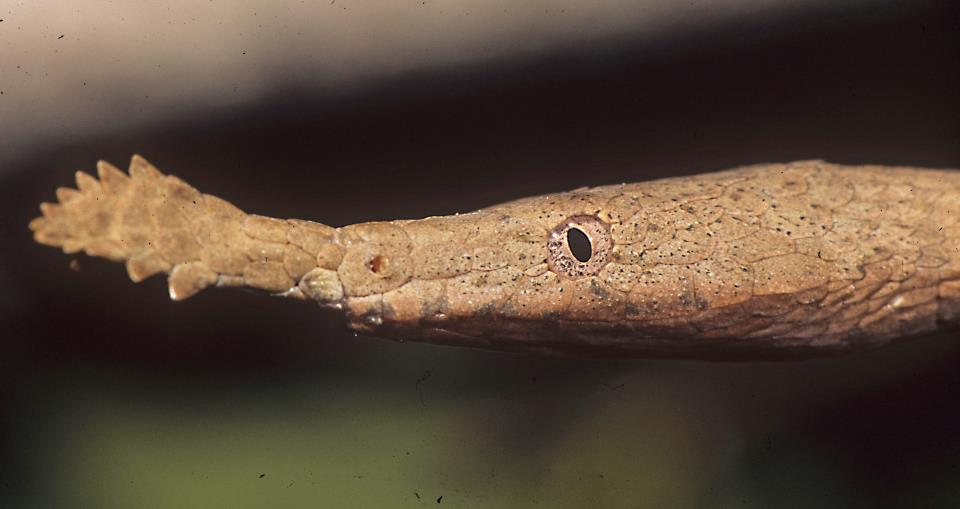
Example dataset: Malagasy Leaf-nosed Snake (Langaha madagascariensis)
Sticking with the snake theme we will look at occurrence data for the genus Langaha, a monotypic genus endemic to Madagascar. The Malagasy Leaf-nosed Snake Langaha madagascariensis is the sole species within this genus and it displays a striking (and yet to be explained) sexual dimorphism.

A quick note about citations
GBIF data should be cited when used in reports, publications, or assignments. The proper citation format for GBIF data used in this exercise is:
GBIF.org (16 September 2026) GBIF Occurrence Download https://doi.org/10.15468/dl.y98fz3
1. Import packages
We will use pandas for table cleaning and geopandas for mapping points.
The data file is a GBIF occurrence download. Even though the file ends in .csv, it is tab-delimited, so we will use sep=" " when we read it.
import pandas as pd
import geopandas as gpd
2. Load the occurrence records
Start by reading the file and looking at the first few rows. The original file has many columns because GBIF exports a lot of metadata with each record.
# GBIF data is tab-separated by default so we need to this to pandas with: `sep="\t"`
langaha = pd.read_csv("Langaha/Langaha-Occurrences.csv", sep="\t")
langaha.head()
3. Inspect the size of the dataset
Before cleaning data, always ask how many rows and columns you have. This gives you a baseline for later, when records are removed by cleaning steps.
langaha.shape
4. Look at the column names
GBIF data can feel overwhelming because there are many columns. Looking at the column names helps us decide which fields are useful for this lab.
langaha.columns
5. Keep a smaller set of useful columns
For this lab keep columns related to identity, location, date, record type, and GBIF data quality flags.
Reducing the number of columns makes the table easier to inspect while we learn the cleaning workflow.
Remember: Pandas dataframes are tables with one row per record and one column per metadata field. You can subset a dataframe by passing in a list only the column names to keep, which is what we do in the next cell.
columns_to_keep = [
    "gbifID",
    "occurrenceID",
    "genus",
    "species",
    "scientificName",
    "countryCode",
    "stateProvince",
    "locality",
    "decimalLatitude",
    "decimalLongitude",
    "coordinateUncertaintyInMeters",
    "eventDate",
    "year",
    "basisOfRecord",
    "institutionCode",
    "collectionCode",
    "catalogNumber",
    "issue",
]

langaha = langaha[columns_to_keep]
langaha.head()
6. Make a simple cleaning log
As we clean the data, we will record how many records remain after important steps. This is a good habit because it makes your workflow easier to explain later.
cleaning_log = []

cleaning_log.append({"step": "raw records", "n_records": len(langaha)})
pd.DataFrame(cleaning_log)
7. Check taxonomic names
Before mapping or filtering coordinates, check which species names are present. This dataset is for the genus Langaha, but it includes more than one species name.
langaha["species"].value_counts(dropna=False)
# Get a list of True/False per row based on whether the record is L. madagascariensis
is_madagascariensis = langaha["species"] == "Langaha madagascariensis"

# Filter the dataframe on these species ID boolean values
langaha = langaha[is_madagascariensis]

# Update the cleaning log
cleaning_log.append({"step": "only L. madagascariensis", "n_records": len(langaha)})
pd.DataFrame(cleaning_log)
8. Check record types
The basisOfRecord column tells us what kind of occurrence record each row represents. Examples include preserved specimens and human observations.
Different analyses may use different record types, so it is useful to inspect this column early.
langaha["basisOfRecord"].value_counts(dropna=False)
9. Check country codes
Langaha is endemic to Madagascar. Madagascar has the country code MG in GBIF.
If we see records from other countries, those records need closer inspection.
langaha["countryCode"].value_counts(dropna=False)
10. Convert coordinate columns to numbers
Sometimes coordinate columns are read as text, especially when files contain missing values. pd.to_numeric() makes sure Python treats these columns as numbers.
The option errors="coerce" turns values that cannot be interpreted as numbers into missing values.
langaha["decimalLatitude"] = pd.to_numeric(langaha["decimalLatitude"], errors="coerce")
langaha["decimalLongitude"] = pd.to_numeric(langaha["decimalLongitude"], errors="coerce")
langaha["coordinateUncertaintyInMeters"] = pd.to_numeric(langaha["coordinateUncertaintyInMeters"], errors="coerce")
langaha["year"] = pd.to_numeric(langaha["year"], errors="coerce")

langaha[["decimalLatitude", "decimalLongitude", "coordinateUncertaintyInMeters", "year"]].head()
11. Find records with missing coordinates
Records without latitude or longitude cannot be mapped directly. They may still be useful for some questions, but they are not useful for point-based spatial analysis.
missing_coordinates = langaha[
    langaha["decimalLatitude"].isna() | langaha["decimalLongitude"].isna()
]

missing_coordinates.shape
12. Remove records with missing coordinates
Create a new table called langaha_clean. From this point on, we will apply cleaning steps to this copy rather than repeatedly changing the original raw table.
langaha_clean = langaha.dropna(subset=["decimalLatitude", "decimalLongitude"]).copy()

cleaning_log.append({"step": "removed missing coordinates", "n_records": len(langaha_clean)})
pd.DataFrame(cleaning_log)
13. Check global coordinate ranges
Latitude should be between -90 and 90. Longitude should be between -180 and 180.
This catches impossible coordinate values. It does not catch all bad records, but it is a useful first check.
valid_global_coordinates = (
    langaha_clean["decimalLatitude"].between(-90, 90)
    & langaha_clean["decimalLongitude"].between(-180, 180)
)

langaha_clean[~valid_global_coordinates]
14. Keep globally valid coordinates
No single cleaning rule is enough, so we apply rules one at a time and check the number of remaining records.
langaha_clean = langaha_clean[valid_global_coordinates].copy()

cleaning_log.append({"step": "kept globally valid coordinates", "n_records": len(langaha_clean)})
pd.DataFrame(cleaning_log)
15. Map the records before geographic filtering
A map is often the fastest way to notice obvious spatial problems. At this stage, we have removed missing and impossible coordinates, but there may still be records far outside Madagascar.
langaha_gdf = gpd.GeoDataFrame(
    langaha_clean,
    geometry=gpd.points_from_xy(langaha_clean["decimalLongitude"], langaha_clean["decimalLatitude"]),
    crs="EPSG:4326",
)

langaha_gdf.explore(column="species", cmap="rainbow")
16. Check for records outside Madagascar
A simple bounding box is not a perfect range map, but it is useful for flagging obvious errors.
For this exercise, use a broad Madagascar bounding box:
- latitude between -26 and -11
- longitude between 42 and 51
Records outside this box are suspicious for Langaha.
in_madagascar_box = (
    langaha_clean["decimalLatitude"].between(-26, -11)
    & langaha_clean["decimalLongitude"].between(42, 51)
)

# Because `in_madagascar_box` is a True/False list for _keeping_ records within the bounding box we described
# if we want to see records outside this bounding box we can invert the truth values
# of this list with the negation operator (the `~` symbol in front of the boolean array)
langaha_clean[~in_madagascar_box][
    ["gbifID", "species", "countryCode", "stateProvince", "decimalLatitude", "decimalLongitude", "locality"]
]
17. Keep records inside the Madagascar bounding box
This removes obvious spatial outliers for this genus. In a real project, you would document and justify the geographic rule you used.
langaha_clean = langaha_clean[in_madagascar_box]

cleaning_log.append({"step": "records inside Madagascar bbox", "n_records": len(langaha_clean)})
pd.DataFrame(cleaning_log)
18. Check country codes again
After geographic filtering, check whether country codes still make sense. Records inside the Madagascar bounding box should mostly have the country code MG, but some records may have missing or unusual metadata.
langaha_clean["countryCode"].value_counts(dropna=False)
19. Inspect GBIF issue flags
The issue column contains GBIF's data quality flags. Multiple flags are separated by semicolons.
Not every issue means a record must be removed. Some are informational, while others may be serious for spatial analysis.
langaha_clean["issue"].value_counts(dropna=False).head(15)
20. Flag high coordinate uncertainty
Coordinate uncertainty tells us how precise the location is, in meters. A record with uncertainty of 500 m may be useful for many maps. A record with uncertainty of hundreds of kilometers is probably not useful for fine-scale spatial analysis.
For this exercise, flag records with uncertainty greater than 10,000 m (as a demonstration).
The tolerance for uncertainty that you will choose should be informed by the distribution patterns of your organism and the spatial grain of your environmental data. 10Km uncertainty may be fine for a widely distributed species that occupies the great plains of N America, but 10Km of uncertainty for a range-restricted alpine endemic might be too much.
high_uncertainty = langaha_clean["coordinateUncertaintyInMeters"] > 10000

langaha_clean[high_uncertainty][
    ["gbifID", "species", "decimalLatitude", "decimalLongitude", "coordinateUncertaintyInMeters"]
].head()
21. Remove records with very high coordinate uncertainty
Here we remove records with coordinate uncertainty greater than 10 km. Records with missing uncertainty are kept for now, but we should remember that they are not necessarily high-quality records.
langaha_clean = langaha_clean[
    langaha_clean["coordinateUncertaintyInMeters"].isna()
    | (langaha_clean["coordinateUncertaintyInMeters"] <= 10000)
]

cleaning_log.append({"step": "removed uncertainty > 10 km", "n_records": len(langaha_clean)})
pd.DataFrame(cleaning_log)
22. Look for duplicate records
GBIF datasets can contain duplicate records. Here we check for duplicates using exact matches in species, latitude, longitude, and year.
This is a simple deduplication rule. Real projects may need more careful decisions.
duplicate_records = langaha_clean[langaha_clean.duplicated(
    subset=["species", "decimalLatitude", "decimalLongitude", "year"],
    keep=False,
)]

duplicate_records[["gbifID", "species", "decimalLatitude", "decimalLongitude", "year", "basisOfRecord"]].head(20)
23. Remove simple duplicates
Use drop_duplicates() to keep the first record from each repeated species-coordinate-year combination.
langaha_clean = langaha_clean.drop_duplicates(
    subset=["species", "decimalLatitude", "decimalLongitude", "year"]
).copy()

cleaning_log.append({"step": "removed simple duplicates", "n_records": len(langaha_clean)})
pd.DataFrame(cleaning_log)
24. Filter by date
Records without a year may be difficult to use for questions about recent species distributions.
For this exercise, create a recent dataset containing records from 1950 onward. This is just an example threshold; your research question should determine the real cutoff.
langaha_recent = langaha_clean[
    langaha_clean["year"].notna()
    & (langaha_clean["year"] >= 1950)
]

cleaning_log.append({"step": "kept records from 1950 onward", "n_records": len(langaha_recent)})
pd.DataFrame(cleaning_log)
25. Make a final cleaned GeoDataFrame
Now convert the cleaned recent records to a GeoDataFrame. This is the version we would use for a first map or for later spatial analysis.
langaha_recent_gdf = gpd.GeoDataFrame(
    langaha_recent,
    geometry=gpd.points_from_xy(langaha_recent["decimalLongitude"], langaha_recent["decimalLatitude"]),
    crs="EPSG:4326",
)

langaha_recent_gdf.head()
26. Map the cleaned records
Color the records by species to see how the cleaned records are distributed across Madagascar.
langaha_recent_gdf.explore(column="species")
27. Save the cleaned data
Saving the cleaned records makes the workflow reproducible. If you change the cleaning rules later, rerun the notebook and create a new cleaned file.
This writes a CSV file inside the Langaha folder.
langaha_recent.to_csv("Langaha/Langaha-cleaned.csv", index=False)
29. What did we remove?
Look back at the cleaning log. A good data cleaning workflow should make it clear what changed and why.
pd.DataFrame(cleaning_log)
Discussion questions
- Which cleaning step removed the most records?
- Which cleaning step involved the most judgment?
- Would you keep records with missing coordinate uncertainty? Why or why not?
- How might these choices change for a broad-scale range map versus a fine-scale habitat model?
Practice submitting your work to your github
Now that you have run through this exercise, practice submitting your notebook code to your class repo.
Open a terminal window and run these commands to add, commit, and push your notebook:
# Go to the labs directory in the course repo
cd ~/BIO597-SpatialBiodiversity/docs/labs

# Add your changed lab
git add Lab03-DataCleaning.ipynb
git commit -m 'Finished Lab03'
git push